Fit wizard
The current ordinary model’s fixed time response also applies to fresh candidates, null baselines, retries, and dense curves. Recommendations and Apply retain it; response changes invalidate cached analysis identity. A recommendation with a different response cannot be applied; reopen the wizard and analyse again after changing Time response. Pulse settings are supplied context, not extra candidates.
The fit wizard is a guided workflow for choosing a sensible single-spectrum time-domain fit function. Open it, click Analyze, and it fingerprints the active spectrum, screens candidate model families drawn from the component library, ranks the fitted candidates with an information criterion (AICc by default), and hands you a plain-language recommendation with a confidence grade. Accepting it writes the chosen result back into the single-fit tab. The most natural use is the first pass on an unfamiliar spectrum — temperature points in the middle of a transition, a sample whose magnetic structure is not yet known, a survey of multiple compounds in a synthesis batch — but the ranking is also a useful sanity check when you already suspect a model: if the wizard does not agree with your guess, digging into the decision trail usually tells you why. For the very simplest cases (clean single-frequency transverse-field (TF) precession, an obvious single-exponential decay) building the model by hand in the fit panel remains faster.
Once the wizard has written a model into the single-fit tab, Fitting engine covers running and refining it and Assessing a Fit covers judging the result; for the same guided approach applied across a whole run series, see the Global fit wizard.
The wizard opens in a non-modal window from the single-fit tab and does not start the expensive analysis until you press Analyze. It uses the same dataset and bunching that the single-fit tab is using at the time you open it, but it analyses the whole record rather than the plot’s fit range: a heavily damped line lives in the first few tens of nanoseconds, before most fit ranges open, and a slow one needs the late tail, so cropping before looking would answer a different question from the one you asked. Applying a candidate is unaffected — the model and its fitted parameters go to the single-fit tab, which goes on fitting your range. Where that range would exclude a line the recommendation rests on, the wizard says so above the result:
The plot’s fit range starts at 1.2 µs, after the 240 MHz line (1/λ = 0.023 µs) has decayed; widen the range before applying this fit.
Completed wizard analyses are cached per dataset in the fit-panel state, reused when the wizard is reopened on the same run, persisted in project files, and consumed by the Global Fit Wizard as the screening table for ordered-series analysis. Reopening the wizard on a run it has already analysed (with nothing changed) skips straight to the result — no need to click Analyze again.
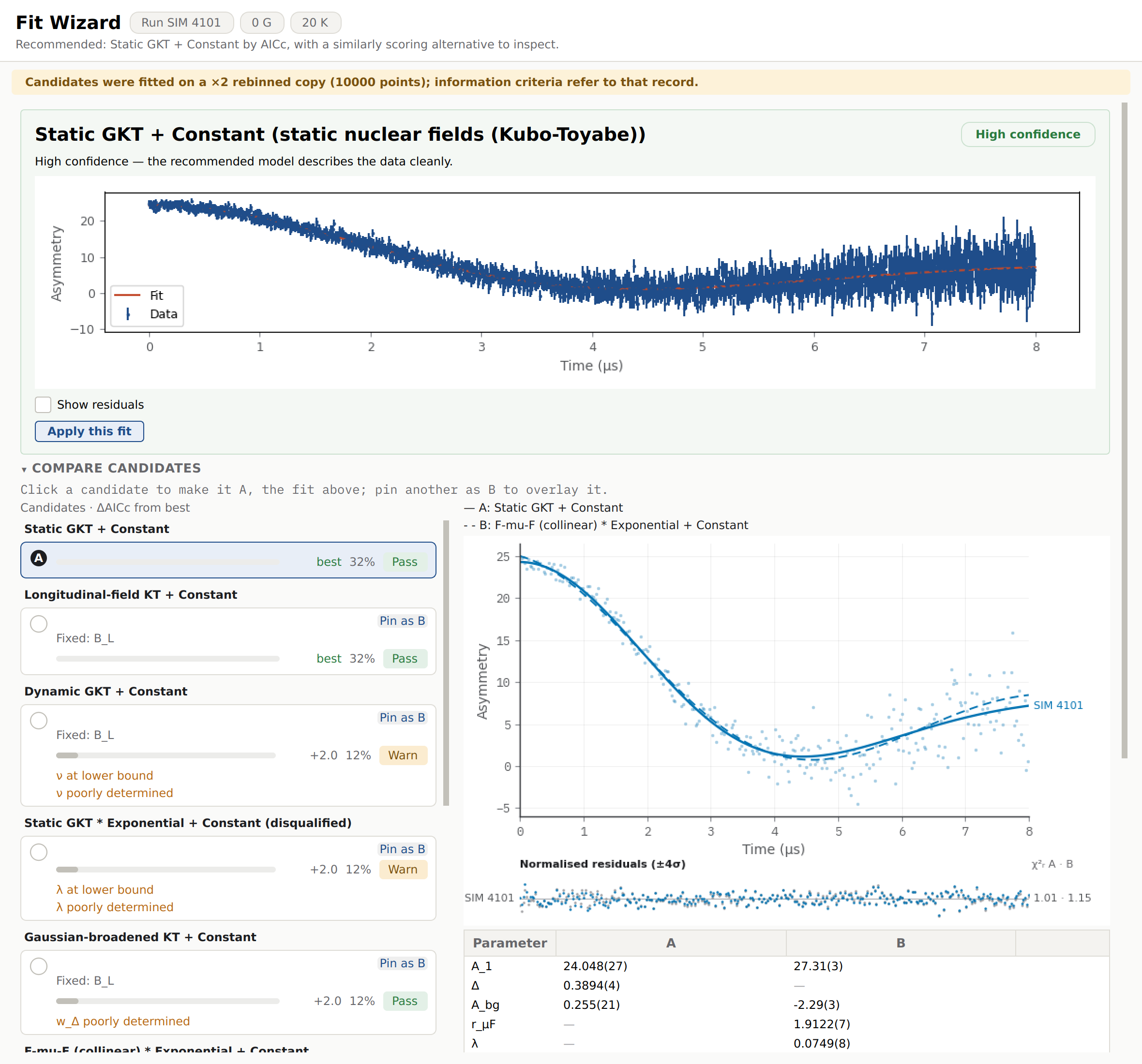
The wizard’s result page on a synthetic ZF Ag polycrystal dataset: the answer card gives the plain-language verdict, a confidence grade, and the data with the recommended fit overlaid. Below it, the Compare candidates section ranks every candidate and sets the recommendation (A) against a pinned alternative (B), above a decision trail whose steps expand to show the reasoning.
The two-click path
For most spectra the whole interaction is: open the wizard, click Analyze, read the answer. Everything else on the page is there for when you want to check the wizard’s working, not because you have to read it first.
Open. The wizard opens on a plain explanation of what it is about to do — analyse this spectrum, fit a set of physics-motivated candidate models, and recommend one with a confidence grade, typically in about a minute — with the run number, field, temperature, and sample beside the title. Below it sits the model family picker (see Choosing which models to screen), which you can leave as it is.
Analyze. Click the Analyze button. There is no surprise computation before this point.
Watch the decision trail. While the analysis runs, a short list of stage headlines lights up one at a time as the wizard works through reading the run conditions, choosing physics families, searching the spectrum, fitting candidates, and weighing the winner. Cancel stays visible the whole time. The status line says you “can keep using the main window while recommendations are prepared”, and you can: if the main window ends up in front, the wizard returns to the front by itself as soon as the analysis finishes.
Read the answer card. When the run finishes, the wizard shows an answer card: a plain-language verdict headline, a confidence sentence, a plot of the data with the recommended fit overlaid, and a prominent Apply this fit button. A “no significant structure” result is shown here as a legitimate outcome, not an error.
Apply, or dig in. Click Apply this fit to hand the candidate to the single-fit tab. To weigh it against the other candidates first, use the Compare candidates section below the card (see Comparing candidates and applying a fit); to see the reasoning, expand any step of the decision trail beneath it.
Choosing which models to screen
Both the wizard’s running time and its answer depend on which candidate models it screens. Screening every model in the component library is safe but slow — a few numerically integrated models dominate the time — and a model that cannot describe your experiment only adds a chance of a spurious winner. The model family picker, shown open on the welcome page above Analyze, sets that list. Leave it as it is and the wizard screens every model that applies to the run; the same picker drives the Global fit wizard.
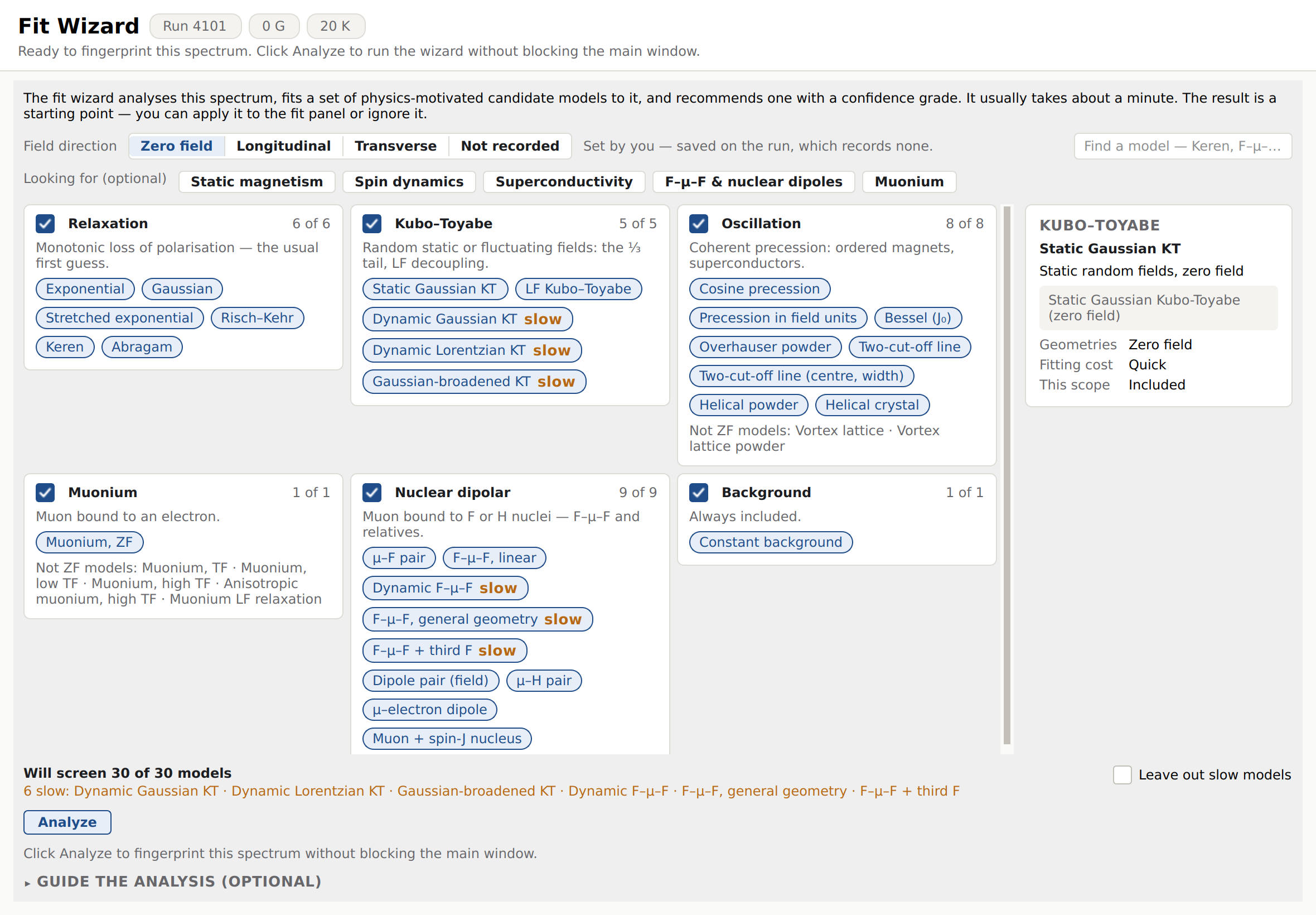
The welcome page on the synthetic ZF Ag run. The file records no field direction, so the direction was answered “Zero field”, and the TF- and LF-only models are listed under their cards as not applying. The details panel shows the static Gaussian Kubo–Toyabe model, and the footer names the six slow models still in the screen.
From top to bottom, the picker holds:
Field direction. Which models apply depends first on the applied-field geometry, and the wizard reads it from the data file only — it never guesses a direction from the field magnitude. When the file records one, the row simply states it (“Recorded: Longitudinal”, for example). When it records none, as PSI ROOT files and synthetic runs often do, the note reads “The run records no field direction.” and every geometry is screened, which is the slow path. Answering Zero field, Longitudinal, or Transverse narrows the screen to that geometry’s models. The answer is saved on the run (“Set by you — saved on the run, which records none.”), kept in the project file, and re-applied when the project is reopened; it never overrides a direction the file records, and if a later file does record one, the file wins. Not recorded withdraws the answer. The answer matters beyond the screen: a Longitudinal answer lets the wizard hold \(B_L\) at the recorded field instead of fitting it (see The applied field is not a fitted parameter). A transverse- or longitudinal-field run whose setpoint is within 2 G of zero also screens the zero-field models, and at a known transverse field the muonium forms outside their validity regime are left out (the low-TF doublet above ~150 G, the Paschen-Back pair below ~1.5 kG; the exact four-frequency muonium model is never field-excluded).
Looking for (optional). Five chips name the physics you expect: Static magnetism, Spin dynamics, Superconductivity, F–μ–F & nuclear dipoles, and Muonium. With none selected every class is screened. Selected chips combine, so a longitudinal-field run can be screened for spin dynamics and muonium together. Generic relaxation and the constant background are always included.
Family cards. One card per family — Relaxation, Kubo–Toyabe, Oscillation, Muonium, Nuclear dipolar, and Background, plus Your functions when you have registered User functions. Each card has a checkbox that switches the whole family on or off, a count of its models in the screen (“5 of 5”), a one-line description of the family, and one pill per model that applies, which you click to switch that model on or off. A slow tag marks the models whose screening fits are expected to take more than 5 s per run on this computer (see which models are slow). Models that do not apply to the run are listed under the card rather than hidden — “Not ZF models: …”, or, at a known transverse field, “Outside these runs’ field range: …”.
Search. The box beside the direction row (“Find a model — Keren, F–μ–F, helix…”) matches a model’s readable name, its registry name, and its one-line use; matching pills are outlined and the rest dimmed.
Details panel. Hovering or clicking a pill shows what that model is for: its name and one-line use, the component description, the Geometries it applies in, its Fitting cost on this computer (below), and under This scope either “Included” or why it is out (for example “switched off by you”). A narrow window hides the panel; each pill’s tooltip still says what the model is for.
Footer. “Will screen N of M models” counts the included models out of those that apply to the run, and the line beneath names the slow ones still included. Leave out slow models drops them in one step. Once you have switched individual models on or off, Reset to suggestions appears; it discards those choices but keeps the chips and the slow switch. With nothing but the background left, the footer reads “Only the background is included — switch on a model to screen.” and Analyze stays disabled.
Which models are slow. How long a model takes to screen depends on its
fits, not on the cost of one evaluation: dynamic Gaussian KT is cheap to
evaluate but slow to fit. The wizard therefore times every candidate fit it
runs. After each analysis it records, for each model, the fit time per 1000
fitted points, taking the median over the candidates that contain the model.
Asymmetry keeps each model’s last nine records in fit_times.json in its
application data folder, and takes their median as the model’s rate. A model
is slow when that rate, scaled to the length of the runs in front of the
picker, comes to more than 5 s per run. The length is the record as the
wizard fits it: a record of more than 8192 points is rebinned first, and a
series uses its median run length. The details panel shows the estimate
(“Slow — ≈ 12 s per run on this computer” or “Quick — ≈ 0.4 s per run on
this computer”), and the picker updates as soon as an analysis finishes.
Until a model has been timed on this computer, its declared cost decides and the panel reads “Slow (not yet timed on this computer)” or “Quick”. Nine built-in models start as slow: the two vortex-lattice models, anisotropic high-TF muonium, dynamic Gaussian and Lorentzian KT, Gaussian-broadened KT, and the dynamic, general-geometry and third-F F–μ–F models. The constant background is never timed and never slow. Leave out slow models leaves out exactly the models tagged slow. The timings belong to the computer, not to the project. They never enter a project file, and every project on the computer shares them. If the file is damaged, Asymmetry logs a warning and starts it again.
After an analysis the picker moves into the first step of the decision trail (below), where it shows the scope the result was screened under.
Seeding a peak (optional)
Below the picker, a collapsed “Guide the analysis (optional)” section holds peak seeding. Leave it closed unless you know of a line the automatic search may miss. Inside, the same time-domain and FFT plots you would see after analysis are already available, so you can seed a peak before the first run. Clicking on the FFT plot adds a user peak at that frequency (dashed red marker); clicking an existing user marker removes it. A peaks table lists every seeded and already-detected line and supports the same removal from a selected row. User peaks are treated as trusted frequencies: they seed oscillatory candidates directly and participate in pattern matching, which is the quickest way to steer the wizard when you can see a line it underrates. Naming a frequency also buys you its envelope: the same Δχ² test the damped-line scan uses is run at the frequency you clicked, and the rate it measures appears in the peaks table’s “Damping (µs⁻¹)” column and seeds the oscillator’s envelope. Because you supplied the frequency, the test no longer has to correct for having searched a whole band, so a line the blind scan declined can still be measured this way; a click on empty spectrum measures nothing and the seed stays a bare frequency. A heavily damped line that the windowed FFT plot cannot show you no longer needs seeding by hand at all — see Heavily damped lines: the matched-apodisation scan.
Changing the picker (including the field direction) or the peak seeds after an analysis has already run marks the displayed result stale — a banner says so, and the Analyze button relabels itself Re-run Analysis until you click it again.
The decision trail
Below the Compare candidates section sits the decision trail: six plain-sentence steps summarising how the wizard reached its recommendation. Each step expands to more detail; three of them expand into the same interactive panels you can reach from the welcome page, now populated with the finished analysis:
Run conditions read — the field geometry the screen used, from the file or your answer (or a note that none was recorded, so every family was considered). Expands to the model family picker described above, which moves here from the welcome page; editing it marks the result stale.
Physics families considered — which candidate families were screened and whether each was expanded for detailed fitting.
Spectral search results — how many spectral lines and recognised patterns (a Larmor line, a muonium doublet, an F-μ-F triplet, and similar) were found. Expands to the FFT plot and peaks table, with the same click-to-seed/click-to-remove peak controls available during guidance.
Candidates fitted, rejections with reasons — how many candidate models were fitted successfully, how many reference baselines were also fitted, and, in plain terms, why any candidate was rejected. Expands to the full comparison table (score, information-criterion values, residual-gate status, reduced chi-squared, and parameter count for every candidate; selecting a row makes it candidate A, exactly as clicking it in the Compare candidates section does).
Winner vs null baseline and checks — the recommended candidate and whether it is decisively better than a plain-relaxation reference.
Confidence statement — the same confidence sentence shown on the answer card, with any caveat spelled out in full underneath.
Expanding a step never re-runs anything; the trail (and every panel it exposes) is derived directly from the completed analysis.
The comparison table (reached from step 4) also lets you switch the ranking metric. A “Ranking metric” control on the result page reranks the already computed candidate fits immediately — it does not rerun the expensive fitting stage. Each shortlisted candidate was fitted with a deterministic multi-start strategy: five initial parameter sets around heuristic starting values, including factor-of-two perturbations, keeping the best successful result per template. The three available metrics are:
Here \(k\) is the number of free parameters and \(n\) is the number of
fitted points. Smaller values are preferred. AICc is the default because
it adds a small-sample correction when \(n\) is not large compared with
\(k\). It is unavailable when \(n-k-1\leq0\) or the fitted point
count is unknown; such a candidate is excluded from ranking under AICc. Another
metric is never substituted. Fixed parameters, link followers and tie followers
do not count toward \(k\); free auxiliary tie parameters do. If no row is
rankable, the message is “No candidate could be ranked by AICc; inspect
unavailable criteria and fit diagnostics before applying a model.”
Unavailable cells show “—”. Hover for the reason and recorded counts, for
example “AICc undefined: n − k − 1 = 0 (n = 4 points, k = 3 free parameters)”.
The CLI screening table prints n/a; its JSON candidate rows contain
aicc: null and an aicc_unavailable explanation.
The correction is derived for linear Gaussian models with an estimated variance and is used here as the conventional small-sample correction [aicc_primary]. Comparisons require the same data and likelihood; a data-only additive likelihood constant cancels only under that condition. AIC is due to Akaike [aic_primary] and BIC to Schwarz [bic_primary].
The scriptable InformationCriteria value records only the finite
\(-2\ln L\), free-column count and fitted sample count. Its value and
unavailable_reason methods expose availability; rank returns both the
ranked and excluded candidates, with reasons. A saved wizard recommendation
recomputes its criteria from its fit statistics and cannot publish an undefined
score as its recommendation.
BIC applies a stronger penalty to model complexity and therefore usually
favours simpler descriptions.
Comparing candidates and applying a fit
A recommendation is only as good as the alternatives it beat, so the result page lets you set any candidate beside it. The Compare candidates section below the answer card is the same comparison panel the Global Fit Wizard uses in its Compare step (see Global fit wizard), here with a single run.
On the left, every candidate the wizard fitted is listed best first (the
caption names the ranking metric, “Candidates · ΔAICc from best”), including
the reference baselines and any disqualified candidate, marked “(baseline)”
and “(disqualified)”. Each row carries a bar for its difference from the best
candidate on the ranking metric, its evidence weight — the Akaike weight
\(w_i \propto \exp(-\Delta_i/2)\) normalised over the list, read as a
percentage — a Pass or Warn badge for the residual checks, with any
failing check spelled out beneath, a “Fixed:” line naming parameters that
were held fixed, and parameter flags (“at lower bound”, “at upper bound”,
“not finite”, or “poorly determined”).
Click a row to make it candidate A. A starts as the recommendation, and A is what the answer card draws and what Apply this fit hands off: picking another candidate here redraws the card’s plot with that candidate’s fit and titles it with the candidate’s name. Pin as B on any other row overlays it as candidate B, and Unpin B clears it. On the right, the data are drawn with A solid and B dashed, above a strip of normalised residuals \((y - f)/\sigma\) (A in colour over B in grey, clipped at \(\pm4\sigma\), with each candidate’s \(\chi^2_\nu\) at the end, “χ²ᵣ A · B”). Below, a parameter table sets A’s fitted values beside B’s, with a note column for either side’s parameter flags. The wizard draws the fitted curve only for the candidates it answers with; the first time you pick any other candidate as A or B, its curve is built in the background and appears a moment later, while the data are shown straight away. Apply A to the fit panel at the foot of the section applies A, as Apply this fit does.
A “Show residuals” toggle under the card’s plot switches it to a residuals view for A.
Applying a candidate (from the card or from the Compare candidates section) updates the single-fit tab: the composite function is replaced with the chosen candidate, fitted parameter values are written into the parameter table, the fit summary is updated with the wizard statistics, and the rest of the GUI refreshes normally. Even if you do not apply a candidate immediately, the comparison table is preserved with the analysis; this matters for later global analysis, because the Global Fit Wizard can reuse the stored per-run tables instead of recomputing them.
If you want to reconsider from scratch, Re-analyze returns to the opening page so you can adjust the picker or the peak seeds before running again — this is a different action from Re-run Analysis, which is what the Analyze button relabels itself to after a picker or peak-seed change makes the current result stale.
Copy analysis log renders the full six-step decision trail — headline and detail bullets for every step — as plain text to the clipboard. This is the right thing to paste when asking a supervisor to sanity-check a recommendation, or when reporting an issue with the wizard: it captures exactly what the wizard considered and why, without requiring a screenshot.
Candidate families
The wizard groups the component library into families — simple relaxation, multi-rate relaxation, static nuclear fields (Kubo-Toyabe), precession signals (including vortex-lattice line shapes), muonium, and muon-fluorine bonding (μ-F / F-μ-F) — and screens them in two stages. Stage 1 fits one cheap representative per in-scope family (both exponential and Gaussian shapes for the relaxation family). A family is expanded to its full portfolio when its representative passes the residual checks, scores within a small margin of the best family, matches a recognised multiplet pattern in the detected peaks, or is pointed at by a fingerprint hint — and an accepted matched-apodisation scan line promotes the oscillatory family the same way a pattern match does. Expensive members such as the numerical F-μ-F powder averages are only ever fitted inside an expanded family, seeded from the match (a hyperfine constant from a muonium pair, a μ-F distance from a triplet). When several strong spectral lines are detected, the wizard also constructs multi-cosine candidates with one damped oscillator per line, up to three.
The applied field is not a fitted parameter
Two parameters in the component library describe the field you applied rather
than anything the sample did: field, the transverse field the muonium and
vortex-lattice line shapes precess in, and B_L, the longitudinal component
carried by the Kubo-Toyabe family (LongitudinalFieldKT,
DynamicGaussianKT, DynamicLorentzianKT, GaussianBroadenedKT,
Keren) and by MuoniumLFRelax. Both are recorded in the run metadata, so
the wizard seeds them from it and holds them fixed. Fitting a quantity you
measured on the magnet costs a degree of freedom in every information criterion
and buys nothing.
For B_L the rule follows the recorded geometry, because a magnitude alone
does not say how much of the field lies along the muon spin:
a zero-field run pins
B_Lat 0, whatever magnitude the file carries. AZFlabel means the magnet was nulled; a non-zero setpoint recorded beside it is a nominal or stale reading, not a longitudinal field;a longitudinal-field run with a recorded setpoint pins
B_Lat that setpoint — including a run whose file records no direction but which you answered Longitudinal in the model family picker;a field magnitude of zero (within 0.1 G) pins
B_Lat 0 in any geometry, recorded or not — a zero applied field has a zero longitudinal component however it is oriented;a transverse setpoint, or a run whose field was never recorded, leaves
B_Lfree. It is then seeded at a small positive field rather than at its zero lower bound: Minuit cannot start a parameter sitting on a limit, and a seed inside the decoupling window (\(\omega_0 < 0.05\,\Delta\), where the Kubo-Toyabe functions use their exact zero-field form) would leave the fit with no gradient inB_Lat all.
The zero-field case is the one that used to bite. B_L was seeded but left
free, so on a genuine zero-field record it started exactly on its own lower
bound, the fit came back “parameters at limit, EDM above threshold”, and the
wizard discarded the record’s own model in favour of whatever shape merely
fitted — a stretched exponential, typically, and with High confidence.
One consequence is worth knowing when you read the comparison table. With
B_L pinned at 0, LongitudinalFieldKT + Constant is the same function as
StaticGKT_ZF + Constant fitted on the same three free parameters, so the two
score identically. The wizard recommends the one that never carried the pinned
extra and shows the other as a similarly scoring alternative.
Pinning an LF setpoint is deliberately a hard pin and not a window around the
recorded value. A magnet calibrated wrongly enough to matter is a hardware
problem the fit should not quietly absorb into B_L: the fix is to correct
the metadata, or to untick Fix for B_L in the single-fit tab after
applying the candidate, which the wizard leaves ticked exactly so you can see
what it decided.
Heavily damped lines: the matched-apodisation scan
An oscillation whose envelope dies in the first few tens or hundreds of
nanoseconds lives entirely in the leading fraction of the record — and every
symmetric apodisation window (hann, cosine, gaussian) is zero at
the first sample, so a windowed transform deletes it. That is the same trap
the library’s ApodisationEarlySignalWarning
exists to flag when you drive the Fourier tools yourself.
The wizard’s spectral search therefore runs a second, unwindowed pass: a matched-apodisation scan. The record is multiplied by a decaying exponential \(e^{-t/\tau}\) and transformed, once for every \(\tau\) on a geometric ladder running from about twenty time bins up to half the informative record, at roughly four rungs per decade. A line whose own envelope is \(e^{-\lambda t}\) reaches its greatest signal-to-noise on the rung where \(\tau = 1/\lambda\), because the apodisation is then a filter matched to the signal — the classical result that, for a known pulse shape in additive noise, the filter matched to that shape maximises the output signal-to-noise ratio. The rung a line peaks on therefore measures its damping instead of inferring it from a crop length somebody chose, and no crop is asked of you: the ladder replaces it. Detection runs on the whole record, truncated only at the point where the growing per-point error has made the remaining data uninformative.
A peak on the ladder is a candidate, not a line. Each candidate is tested by weighted linear least squares: the record is fitted with a dictionary of slow decays (\(e^{-\lambda_k t}\) for \(\lambda_k\) = 0, 0.3, 1, 3, and 10 μs-1), then again with an \(e^{-\lambda t}\cos\) / \(e^{-\lambda t}\sin\) pair added at the candidate’s \((f, \lambda)\), and the χ² improvement Δχ² between the two is maximised over a bounded box around the seed. Both fits are linear, so Δχ² is exact rather than the outcome of an iterative search. Acceptance is a look-elsewhere-corrected threshold,
where \(r\) = 0.01 is the number of false lines tolerated per record and \(N_\mathrm{trials}\) counts the independent cells the ladder searched — the same philosophy as the windowed pass’s SNR gate, applied to a statistic rather than to an amplitude ratio. An accepted line joins the nuisance basis and is subtracted from the record before the ladder is scanned again, so a strong line’s skirt cannot manufacture a second one; up to three lines are found this way, each finally re-fitted with the others held in the basis so their reported numbers are comparable.
One accepted line is enough to build candidates the earlier portfolio could not offer: a sum of damped oscillators, one per scan line and up to three, plus a slowly relaxing term and a constant, with either an exponential or a Gaussian envelope on the oscillators. A heavily damped line almost always sits on a relaxing background it decays into, and without a term for that background the fit spends an oscillator on it. Every oscillator is seeded from the measurement — frequency, envelope rate, amplitude, and phase — with rate bounds always containing \(\lambda/4\) to \(4\lambda\) and frequency bounds a few line widths wide. An accepted line also promotes the oscillatory family for detailed fitting, so these candidates are fitted whenever the scan finds anything at all; on a record where it finds nothing they never appear.
Three things to know when reading the result:
Scan lines are labelled
damped_scanin the peaks table, and the envelope each one measured appears in its own “Damping (µs⁻¹)” column, with the amplitude, phase, and Δχ² in the row’s tooltip. On the FFT plot they carry a dashed marker and name themselves in the legend, “Matched-apodisation scan line — not expected to be visible in this windowed transform”: the plot is the windowed transform, so a scan line is legitimately absent underneath its own marker. (The older unwindowed crop ladder, whoseearly_fftpeaks used a dotted marker, remains in the library but no longer runs as part of the search.)Its numbers are not comparable with the windowed pass’s. A scan signal-to-noise is an excess over one rung’s own median-absolute-deviation noise floor, not a magnitude ratio, and Δχ² is a third scale again. Rank peaks within a pass, never across.
Slow lines belong to the windowed pass. Where a line is visible to both, the windowed pass wins: it looked at the whole informative record, so its frequency estimate is the better one, and the scan only ever adds lines the windowed pass missed. The scan is also deliberately blind to slow, low-Q features: a candidate completing fewer than about three cycles inside its own fitted lifetime is read as a relaxation shape rather than an oscillation and rejected, unless its envelope is faster than any relaxation the slow-decay dictionary models. That rule is what keeps a static Kubo-Toyabe minimum out — a single dip and recovery that no sum of monotonic decays reproduces, and which Δχ² alone would happily call a line.
The scan reaches envelope rates of a few hundred μs-1 on a finely binned record. The limit is the short end of the ladder, so what it can reach depends on the binning: 0.1 ns bins reach far further than 16 ns ones. Faster than that the oscillation is not recoverable at any apodisation, and the wizard simply offers no damped candidate. At the other end, a component so overdamped that it barely completes a cycle is fitted as one broad line if it is accepted at all; treat the frequency it reports as a description of that line shape rather than as a precession frequency, and check the fit overlay before reading physics into it.
The additive multi-component candidates are especially useful for spectra whose smoothed semilog envelope changes slope while remaining largely monotonic. In that situation a very low-frequency FFT peak can be a by-product of envelope shape rather than genuine precession, so the wizard distinguishes resolved oscillations from multi-rate monotonic relaxation and can try mixtures of exponential and Gaussian channels with up to three relaxing components.
If the single-fit tab already has a different composite model selected, the wizard fits that function too and keeps it as a baseline comparison, useful when you already have a hand-built function and want to see whether the wizard’s simpler portfolio explains the same spectrum comparably well.
Recommendation rules
The wizard does not claim that there is always one unquestionable winner. Its default recommendation policy is:
Rank successful candidates by the selected metric, excluding null baselines and any candidate disqualified for a targeted physical reason (see Confidence and verdicts below).
Break ties by preferring fewer free parameters.
Break remaining ties by preferring fewer additive terms.
If the top two candidates are within 2 score units, present them as a comparable pair (both have near-equal evidence weights in the Compare candidates list) and recommend the simpler one.
Check the winner against a simpler null baseline. If it does not clear that bar, recommend the null instead.
Otherwise recommend the winner, with a confidence tier set from the residual gate.
This keeps the default behaviour interpretable and favours models that are good enough without adding unnecessary physical parameters.
Confidence and verdicts
Every recommendation carries a confidence tier and, in the unusual case that nothing in the portfolio is worth recommending, a different kind of verdict altogether. Both are stated in plain words on the answer card, and the same wording appears (with any caveat spelled out in full) in the decision trail’s confidence step.
High confidence reads “High confidence — the recommended model describes the data cleanly.” It means the recommended candidate’s residuals pass every check in the residual gate — nothing about the fit’s mismatch with the data looks structured.
Medium confidence reads “Medium confidence — this is the best model tried, but the fit leaves patterns in the residuals. Usable; review before publishing,” followed by a caveat naming which diagnostics still show structure. It means the candidate is still the clear winner by the selected metric, but one or more residual diagnostics still show structure. Treat a Medium-confidence recommendation as usable with that caveat in mind — check the named diagnostics in the residuals view before trusting the fit for publication. Either way, High or Medium, the best-scoring candidate is recommended: the residual gate no longer removes a candidate from consideration, it only tells you how much to trust the number at the top.
What does remove a candidate from consideration is a targeted disqualifier — a check aimed at a specific, physically implausible failure mode rather than general residual shape:
a fitted oscillation frequency sitting at the 1/T resolution floor of the fit window, or pinned against one of its bounds — both are signs the “line” is really an artefact of a too-short window or an unconstrained fit, not a resolved frequency
an oscillation amplitude statistically consistent with zero — the component is present in the model but not actually needed by the data
a free-running oscillation frequency with no supporting line in the detected-peaks table and too few cycles inside the statistically informative part of the window to stand on its own
a relaxation component the data do not resolve — see Are the components actually resolved? below
A disqualified candidate is still shown in the comparison table (step 4 of the trail), with its title suffixed “(disqualified)” and the specific reason available as a tooltip on that row, but the wizard moves on to the next candidate rather than recommending it.
A recommended oscillation that clears that floor but only just — completing somewhere around two to three cycles inside the informative part of the window — keeps its computed confidence tier, but if its spectral line is also weak or missing from the detected-peaks table, the caveat notes that the oscillation sits at the edge of what the run can resolve and suggests a longer or higher-statistics measurement to confirm it. A strong, well-corroborated line at the same cycle count is not flagged.
Before settling on a winner among the surviving candidates, the wizard also checks it against two cheap null baselines that are always fitted unconditionally: a flat constant, and a plain exponential decay plus constant. These appear in the comparison table with their titles suffixed “(baseline)”. If the best candidate does not improve on the simpler of the two nulls by roughly 10 AICc units or more, the wizard concludes that the data do not carry enough structure to justify the richer model and recommends the null baseline instead — this is the wizard’s way of saying “there is nothing here worth a richer model.” The answer card shows this as its own headline, “Your data look like a simple decay — no oscillation worth fitting,” and treats it as a legitimate result rather than a failure: it usually means the spectrum is well described by a plain relaxation (or is flat within the noise), and chasing a more elaborate model would be over-fitting.
Are the components actually resolved?
A composite relaxation model will happily converge with one branch railed to a rate so fast that its 1/e time falls inside the first few time bins, or collapsed so slow that it never decays inside the fit window. Neither is a measured rate: the first is absorbing the leading bins, the second is indistinguishable from a free constant baseline. Both still buy χ², so AICc will “prefer” the extra component — which is exactly how an extra exponential ends up in a published model.
The wizard therefore checks every candidate that carries two or more relaxation rates. For each rate it asks whether the value lies inside the window the data can resolve:
the 1/e time must span at least a few time bins (the fast edge), and
the 1/e time must be no longer than the fit window (the slow edge).
The check is two-sided on purpose. A fast-edge-only rule silently admits the collapsed-to-zero branch, which is the same pathology seen from the other end.
Crucially, the verdict is not read off the fitted value alone. Where the likelihood has a flat ridge in a rate, two optimisers landing in statistically indistinguishable minima can return opposite answers on the same data — one “resolved”, one “railed”. So the wizard judges the whole Δχ² ≤ 1 neighbourhood: it pins the rate just outside each edge, re-fits everything else, and asks whether the data can tell the difference. That gives three distinct outcomes:
resolvedThe rate, and every value the data cannot distinguish from it, sit inside the resolvable window.
unresolved_fast/unresolved_slowThe fitted rate itself is outside the window — railed into the leading bins, or degenerate with the baseline.
undeterminedThe fitted rate is inside the window but the admissible interval reaches outside it. This is the honest third answer: the data do not determine the component either way, and neither “resolved” nor “railed” would be true.
Anything other than resolved disqualifies the candidate, with the reason
carried on the row exactly like the oscillation disqualifiers above.
The same rule is available on its own for scripted analyses, where you can set the bin tolerance your binning justifies and supply your own multistart solutions as the neighbourhood instead of paying for the probe re-fits:
from asymmetry.core.fitting.resolution import assess_component_resolution

assessment = assess_component_resolution(
    fit_result,
    model,
    dataset,
    min_bins_per_e_folding=20.0,      # a rebinned corpus can justify far more
)
if not assessment.is_resolved:
    for reason in assessment.disqualification_reasons():
        print(reason)
Pass solutions=[(chi_squared, {"Lambda_1": ..., "Lambda_2": ...}), ...] to
use converged multistart seeds you already have; pass
probe_neighbourhood=False to fall back to the point estimate, which is
cheapest and documented as optimiser-dependent.
Convergence quality
Comparing two models is only meaningful when both were searched to comparable depth. Two things guard that:
the Stage-2 seed ladder scales with a candidate’s rate dimensionality, so a three-rate family is not judged on the same handful of seeds that fully covers a one-rate family’s search space; the extra seeds widen the seeded rate separation, which is the dimension a multi-component fit exists to determine;
after ranking, the top few candidates are re-fitted with the full seed ladder. Whichever fit is better is the one reported, and the χ² gained is recorded on the assessment as
refinement_delta_chi_squared, withunder_convergedset when it exceeds one χ² unit.
under_converged is not a warning that the reported number is wrong — the
reported number is the deeper fit. It is the measured statement that this
candidate’s original ranking was search-limited, and therefore that the whole
table around it should be read with that in mind. Pass
refine_top_candidates=0 to skip the pass.
A third thing matters on a long record: the candidates are fitted on a rebinned copy of it. A dozen multi-component fits on 105 points is minutes of arithmetic for information a coarser observation already carries, so above roughly 8 000 points the wizard rebins — never so far that the highest seeded frequency drops below eight samples per cycle — and says which record it used:
Candidates were fitted on a ×8 rebinned copy (11250 points); information criteria refer to that record.
Line detection uses its declared spectral observation, retaining the native
bandwidth for captured nonuniform histograms. Candidates fit the selected
rebinned observation. AIC, AICc, BIC, χ²ᵣ, RMS and runs refer to that
fit; a separate residual FFT evaluates the same fitted model and parameters
on the diagnostic observation. Its attribution distinguishes that view from
the original residuals. The recommendation records the fit rebin factor and
point count as rebin_factor and analysed_points.
For a reproducible histogram observation the wizard merges counts and their retained variance before forming asymmetry. It preserves the selected period, projection, alpha/beta, timing, good support, corrections, reference acquisition, and base binning. Toolbar merges compose with the wizard factor once; a cropped input retains its selected output-bin members before further merging. For F = [90, 1] and B = [10, 9], a factor of two gives 65.454545…%, whereas the mean of the two separate asymmetries is 0%.
The captured observation owns read-only copies of sample, held-period, and reference counts and supplied variances, together with copied settings and timing. Editing the original arrays through the scripting API leaves that observation, its cached analysis, and rebuilt curves stable. To analyse edited counts, first reduce them again to capture a new observation, then rerun the wizard.
Curves without resolved histogram context, including custom or historical curves
that retain a Run, and rotated observations use the independent-curve mean.
For conditional calibration errors and histogram Gaussian omission,
see Calibration conditioning and Undefined and degenerate bins.
Used/omitted counts and reasons travel with the core fit result through search,
completion, and rebuilding; model scores count only the fitted observations.
Detection keeps the full acquisition grid. When omission prevents a residual
FFT or acquisition-lag autocorrelation, the diagnostic is unavailable; a valid
fit remains available. No missing-bin interpolation is inserted. The single-run
Details view shows unavailable and the core result explains
Residual autocorrelation and FFT unavailable: Gaussian selection omits acquisition bins.
Historical scores retain their recorded meaning, while numerical reuse requires
the current observation policy.
The wizards still fit asymmetry with conditional Gaussian point errors; TF alpha/beta count calibration is a separate operation. Models are evaluated at the prepared timestamps, so wide bins can attenuate rapid signals.
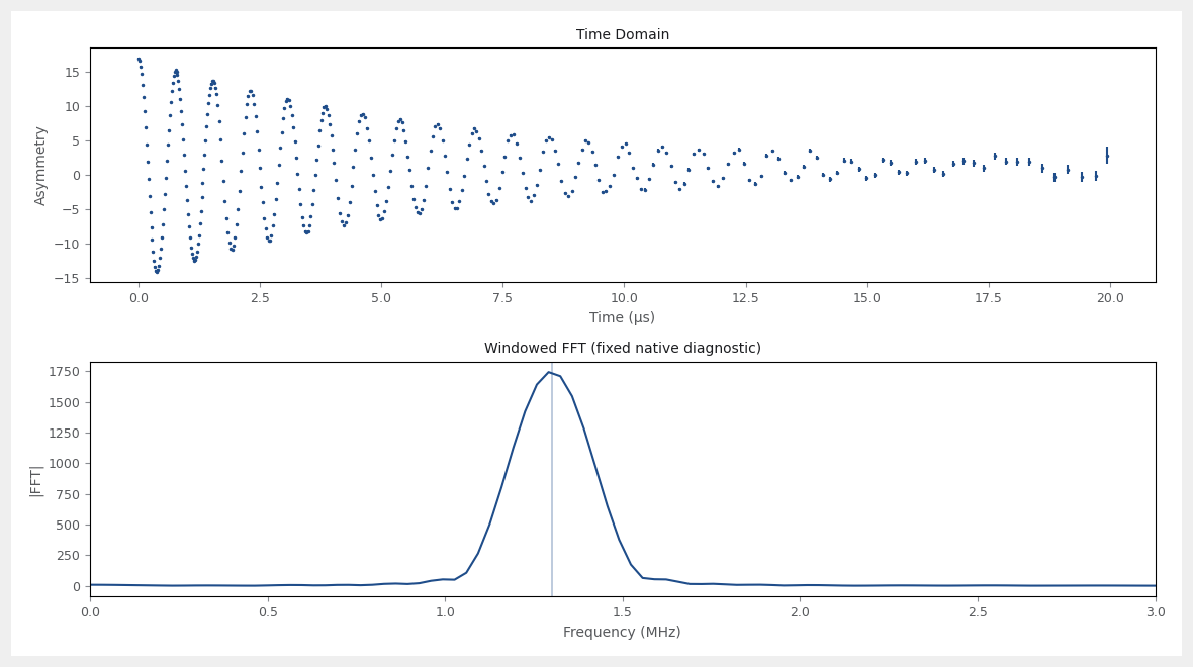
The spectral plot is labelled Windowed FFT (fixed native diagnostic) when a
separate native count view is used. Preparing spectral preview… runs through
the existing cancellable worker preparation; redraws reuse its captured spectrum.
Spectral detection preserves uniform curves. Nonuniform Variable and Constant error histogram observations use a separate Fixed native-bin count reduction (factor 1, merge 1) over exactly their retained native support. Base/toolbar/crop/merge selections are resolved before selecting this grid; incomplete merged tails stay excluded. The captured pair, periods, balances, timing, corrections/reference and retained variances supply the same operation. Hann, early, damped-line and Burg passes share this declared view, whose actual sampling interval and informative window determine spectral bandwidth/resolution. Non-spectral fingerprint features still describe the original science curve. See Fourier analysis for the support rule and direct-FFT sampling limits.
Residual FFTs evaluate the same fitted model/parameters on that separate fixed
count view. The original objective, points, scores, parameters/covariance and
residual times/errors are unchanged; RMS and runs still use original residuals.
The result records separate_fixed_count_reduction when that view is used.
Acquisition-lag autocorrelation is unavailable for nonuniform original residuals.
Omitted Gaussian observations retain the unavailable diagnostic guard above.
Missing diagnostics are not evidence that a model explains the data.
A nonuniform curve-only/custom curve with an attached Run is still refused;
a Run or recipe alone does not establish count replay. Uniform curve-only FFTs
remain supported. A sampled detrend_curve cannot be evaluated on a different
grid; supply detrend_model(time) for a fitted trend. Undefined native ratios
remain unavailable rather than being filled, omitted or averaged into a spectrum.
Defined zero-variance boundary ratios retain Fixed controls’ FFT support and
canonical display errors; Gaussian fit selection remains separate.
Asymmetry also checks that a current assessment’s source observation is unchanged
before rebuilding curves. A changed input raises
Wizard observation changed; rerun the analysis before rebuilding curves.
Rerun the analysis to obtain scores and curves for the edited observation; this
prevents a different record from being drawn under the saved score.
Cached analyses require the same observation, reduction context, selected support, scope, frequencies, numerical preparation contract, and scientific-computation revision. Unknown or older executions cannot supply current reusable recommendations. Rebuilt curves use the same prepared grid as the fitted assessment. Saved historical results retain their values and curve-mean reconstruction semantics; opening them does not refit or relabel their scores.
Compared with other programs
WiMDA 1.326 grouping, musrfit 1.12.1 ordinary packing, and documented Mantid
muon preprocessing combine counts before the F/B ratio. This comparison concerns
input observations, not wizard search or ranking. See Binning and timestamps
for public sources, uncertainty conventions, and matched-support limits.
Mantid 6.16.1 FFT requires linear X coordinates and exposes its shift convention
and full/positive-frequency outputs. musrFT 1.12.1 (708f777b, ROOT 6.40.04)
supports explicit packing and Fourier controls. Matched fixed-grid 1.3 MHz
controls agree within one actual frequency bin; endpoint and amplitude conventions
remain distinct. Neither comparison establishes equivalent wizard ranking or
spectral uncertainties. See spectral conventions.
Calling the wizard from a script
build_fit_wizard_recommendation evaluates its candidate models across a
process pool. Python starts those worker processes with the spawn method,
and every spawn worker begins by re-importing the calling script’s
__main__ module. Put your analysis behind a guard so the workers do not
re-run it:
from asymmetry.core.fitting.fit_wizard import build_fit_wizard_recommendation

def main():
    recommendation = build_fit_wizard_recommendation(dataset)
    print(recommendation.recommended_key)

if __name__ == "__main__":
    main()
Without the guard the wizard detects the situation before starting any worker,
runs serially instead, and warns once with SpawnUnsafeWarning — the
results are identical, only slower. Interactive sessions, python -c ... and
notebooks are unaffected: there is no module for a worker to re-import, so they
keep full parallelism.
Passing max_workers=1 is always a safe escape hatch — it never starts a
worker process at all, and it also makes runs bit-for-bit reproducible when you
need to compare two invocations exactly. The same rules apply to
Global fit wizard, which uses the same machinery.
The returned FitWizardRecommendation carries the record the candidates were
actually fitted on as rebin_factor and analysed_points (both described
under Convergence quality), and its peak_analysis carries
the matched-apodisation scan’s own result — the accepted lines with their
rates, amplitudes, phases, and Δχ², together with the threshold and trial count
they were judged against — as peak_analysis.damped_lines. The scan is also
usable on its own:
from asymmetry.core.fitting.damped_line_scan import detect_damped_lines

analysis = detect_damped_lines(dataset.time, dataset.asymmetry, dataset.error)
for line in analysis.lines:
    print(line.frequency_mhz, line.damping_rate_per_us, line.delta_chi_squared)
measure_line_at_frequency in the same module answers the narrower question
the GUI’s click-to-seed asks: given a frequency you already trust, what is its
envelope?
Limitations
The wizard currently supports one time-domain asymmetry spectrum at a time.
Frequency-domain fingerprinting uses the standard FFT path only; MaxEnt is not part of the wizard workflow.
Analysis and fitting run on the record’s statistically informative window, not necessarily on all of it: where the per-point error has grown to several times its early-time value, the remaining data are noise that would only whiten the transform, so the window is cut there. A run whose errors do not grow that way is analysed whole.
The fit range set in the plot panel governs the fit you apply, not the analysis. A range that would exclude a detected damped line is flagged above the result, not corrected for you.
Information criteria refer to the analysed record, which on a long run is a rebinned copy (see Convergence quality).
max_workersbounds how many fits run at once, not how much CPU the run uses: the vortex-lattice line shapes reach a multi-threaded BLAS from inside a single fit, so evenmax_workers=1can saturate the machine. SetOMP_NUM_THREADS/OPENBLAS_NUM_THREADSin the environment before starting Python if you need to bound it.Recommendations are limited to models that can already be assembled from the supported composite-model components.
Bayesian model comparison is not part of version 1, although the comparison backend is designed so that it can be added later.
The wizard should be treated as a decision aid rather than a replacement for physical judgement. Inspect the fit overlay, residuals, and parameter values before accepting the recommendation, especially when two candidates score similarly.

Sparse Ag control with an authored fixed-background sensitivity operation. The fit keeps usable signed observations; the display retains the full grid. Omission counts and unavailable residual diagnostics belong to the core result.
H. Akaike, IEEE Trans. Autom. Control 19, 716–723 (1974), doi:10.1109/TAC.1974.1100705.
C. M. Hurvich and C.-L. Tsai, Biometrika 76, 297–307 (1989), doi:10.1093/biomet/76.2.297; N. Sugiura, Commun. Stat. Theory Methods 7, 13–26 (1978), doi:10.1080/03610927808827599.
G. Schwarz, Ann. Statist. 6, 461–464 (1978), doi:10.1214/aos/1176344136.