Fourier analysis

Central plot in the Frequency domain showing the grouped Fourier spectrum of a synthetic YBa₂Cu₃O₇₋δ vortex-state TF μSR run (TF = 200 mT, T = 10 K), zoomed to the Larmor peak at γ_μ·B_app ≈ 27.1 MHz. The canonical asymmetric line shape — sharp low-field peak at the saddle-point van Hove singularity, long high-field tail toward the vortex cores — is the textbook signature of an isotropic triangular vortex lattice (Brandt, Phys. Rev. B 37, 2349 (1988); Sonier et al., Rev. Mod. Phys. 72, 769 (2000)).

Fourier analysis answers questions that the time domain answers slowly or not at all: whether a signal contains three precession frequencies or two (multi-site magnets, F-μ-F entanglement, muonium hyperfine pairs), and what the internal-field distribution \(P(B)\) looks like inside the vortex lattice of a type-II superconductor in the mixed state (Superconductor penetration depth from σ(T)). The frequency-domain view is also the standard way to choose a sensible seed frequency before attempting an oscillatory time-domain fit (Oscillation).

Apodisation is the key practical knob. A Lorentzian filter sharpens an exponentially damped line; a Gaussian filter is the natural choice for nuclear-dipolar broadening; None is appropriate only when the signal-to-noise is high enough that the line broadening from apodisation would dominate the intrinsic widths. The panel starts with None selected — choose the filter matched to the expected lineshape rather than leaving the default in place out of habit. Phase correction follows the same logic: the entropy-optimised auto-phase mode is robust for single-frequency signals; for multi-frequency or vortex data, the manual per-group phase table or a future optimised phase fit gives better control. Maximum entropy reconstruction (see Maximum Entropy Method below) is the alternative when an FFT line is too weak or the usable time window too short for the FFT to resolve it.

Note

Apodisation trades resolution for leakage, and the trade is not free. Weighting the time signal down at long times suppresses the spectral leakage (the sidelobes) that a hard truncation would produce, but it also broadens every line: an apodised FFT linewidth is the convolution of the intrinsic width with the filter’s transform, so a width or amplitude read off an aggressively filtered spectrum is not the physical value. Use apodisation to see a line clearly; measure widths and amplitudes with a frequency-domain fit (Frequency-domain fitting) whose model carries the true lineshape, or read them from the time-domain fit directly [6].

Same YBCO vortex-lattice run, same Compute FFT click, three Apodisation settings from the Fourier panel’s controls: the None/Gaussian/Lorentzian radios with Filter τ (µs) set to 4.0 and 3.0 µs respectively. Going from left to right the Larmor peak loses height and gains width — the resolution the filter trades away — while the sidelobe ripple away from the peak flattens out, exactly the resolution-for-leakage trade the note above describes.

Implementation summary

Asymmetry currently exposes two Fourier workflows:

• the core Python API can transform a supplied time-domain dataset directly

• the desktop GUI uses a WiMDA-style grouped-detector workflow that rebuilds a grouped count signal for each included detector group before taking the FFT

In the GUI, the frequency-domain plot transforms one of two signal sources (see Signal source): by default, the average of the currently included groups rather than separate per-group spectra; or, for a single forward/backward detector pair, the run’s forward−backward asymmetry directly. Each loaded dataset keeps its own Fourier phase-table state, so changing runs restores the phase values, included groups, and auto-estimated markers associated with that run.

Notation

In this guide, frequency-domain quantities use standard symbols:

• \(A(t)\) for asymmetry in the time domain

• \(\nu\) for frequency (MHz)

• \(\lvert\mathcal{F}\rvert\) for FFT magnitude

Fast Fourier transform (FFT)

The FFT is the simplest, fastest route to a spectrum: a discrete Fourier transform of the (real) apodised asymmetry, evaluated by the radix Cooley–Tukey algorithm [1] through numpy.fft.rfft(). It is a linear transform, so its amplitudes and areas map directly onto the apodisation settings and can be trusted quantitatively (subject to the resolution/leakage trade above). Asymmetry takes the one-sided real transform and derives every display channel — magnitude, real, imaginary, phase — from that one complex spectrum.

from asymmetry.core.fourier.fft import fft_asymmetry
from asymmetry.core.io import load

dataset = load("data.nxs")

# Compute FFT — returns (frequencies, real_part, magnitude)
frequencies, real_part, magnitude = fft_asymmetry(dataset)

# Plot
import matplotlib.pyplot as plt
plt.plot(frequencies, magnitude)
plt.xlabel(r"$\\nu$ (MHz)")
plt.ylabel(r"$|\\mathcal{F}|$")
plt.show()

Signal source

The Fourier panel’s FFT Phase Mode section starts with a Signal source choice — which time-domain signal is transformed, before any of the apodisation or phase-mode controls below are applied:

• Grouped average (the default) — “Average of each detector group’s lifetime-corrected FFT.” This is the WiMDA-style workflow the rest of this page describes: rebuild each included group’s signal, FFT it, and average the results.

• F−B asymmetry — “FFT of the forward−backward asymmetry signal (as plotted in the time domain) — cleaner for a single detector pair.” Rather than averaging every group’s own FFT, this transforms the single forward−backward asymmetry curve directly — exactly the signal the time-domain plot shows, built with the same grouping and α. Deadtime correction is not applied on this path, matching the time-domain plot (the grouped-average path does apply it to each group’s count signal before the transform).

For a run with just one forward/backward detector pair, F−B asymmetry gives markedly better peak-to-floor contrast than Grouped average: on a real GPS zero-field run, switching to F−B asymmetry raised the contrast by roughly a factor of five, where averaging every detector group’s own FFT buried the line under the other groups’ baselines. With several detector groups, though, Grouped average remains the workflow to use — averaging genuinely independent group spectra is what suppresses their uncorrelated noise.

Switching source flags the displayed spectrum out of date, and the Groups include/phase table becomes inert (and is disabled, not hidden, so the values survive a switch back) in F−B mode, since a single already-combined curve is being transformed — the per-group table cannot affect it. Grouping and α changes still flag the spectrum out of date in F−B mode, because they change the underlying forward−backward curve; the global Phase field and t0 Offset (μs) still apply in the phase-correcting display modes either way. The two sources are also distinguished in overlays: a spectrum computed from F−B asymmetry is labelled <run> F−B rather than <run> Average, so a multi-run overlay’s legend (GUI Fourier workflow) shows at a glance which runs used which source.

Filter / apodisation

The main Fourier workflow now follows WiMDA’s filter model rather than the older whole-trace window presets. The FFT panel exposes three apodisation modes:

• None

• Lorentzian

• Gaussian

along with:

• Filter start (µs)

• Filter τ (µs) — the filter time constant

For a Lorentzian filter, Asymmetry follows WiMDA’s two cases:

\[A_f(t) = e^{-t/\tau} A(t) \qquad \text{when } t_\mathrm{start} = 0\]

\[A_f(t) = \frac{1 + e^{-t_\mathrm{start}/\tau}}{1 + e^{(t - t_\mathrm{start})/\tau}} A(t) \qquad \text{when } t_\mathrm{start} > 0\]

The Gaussian mode uses the same WiMDA-style softened start with squared arguments. Subtract average signal is applied before the filter, matching WiMDA’s default preprocessing path.

Matched-filter suggestion

The Apodisation section’s Suggest from data button estimates the matched filter for the spectrum’s dominant line and fills the fields without applying anything: it selects the filter mode, writes the matched Filter τ (µs) (shown in the green auto-filled colour until you edit it), and reports what it did in the status line —

Suggested Lorentzian τ = 2 µs, matched to the 2.7 MHz line — maximises peak S/N, ≈2× its apparent width.

The out-of-date banner then flags the displayed spectrum, and your explicit Compute FFT applies the filter. Nothing is ever auto-applied: a matched filter maximises the line’s peak signal-to-noise at the cost of roughly doubling its apparent width, which is a trade you should make knowingly — never measure linewidths or moments from a spectrum filtered this way without accounting for it (the spectral-moments readout shows a caveat on apodised spectra for exactly this reason).

The estimate is made from the unapodised power spectrum, whatever the current filter setting: the dominant line inside the field-narrowed search window (the same window automatic phase estimation uses) is measured at half maximum, and the matched time constant follows from the line shape — τ = 1/(πΓ) for a Lorentzian of power-spectrum FWHM Γ, with the equivalent (Dawson-corrected) relation for a Gaussian. If the Gaussian filter mode is selected the match is Gaussian; otherwise Lorentzian.

Detection is two-stage. A cheap check first looks for a line that already towers over the raw spectrum’s noise floor. A line that is genuinely present but sits below that — for example an un-windowed, lifetime-corrected record whose late-time noise is amplified by the deadtime/decay correction — can still be invisible in the raw spectrum while remaining detectable: the fallback search itself smooths the spectrum at a range of candidate linewidths (anchored to the spectrum’s real frequency resolution, not the zero-padded display grid, so it cannot mistake padding-correlated noise for a line), so a line buried in an un-apodised spectrum’s noise floor is still found. “No clear line” now means no line at any scanned width — only then, or when the dominant line is resolution-limited (its width is the transform’s, not the sample’s), does the status read “No clear line to match — leave apodisation off.” and nothing is filled.

How the GUI FFT is built

The docked Fourier workflow in the desktop application is intentionally more specific than the low-level API:

• by default (Grouped average) the FFT input is the grouped detector-count signal, not the forward/backward asymmetry trace; the F−B asymmetry Signal source transforms that asymmetry trace instead

• the grouped signal is rebuilt from the current grouping and current bunching factor every time the transform is computed

• grouped-count inputs are corrected for the muon lifetime envelope before the later mean-subtraction and apodisation stages

• the active time-domain fit range is used as the FFT time window when a fit range is present

• zero padding is applied after the selected time window and preprocessing are fixed

This means the Fourier spectrum shown in the GUI is tied directly to the current grouped analysis state, rather than being a generic transform of whatever line is currently plotted in the time-domain view.

Background subtraction for the FFT input

Because the FFT input is rebuilt from the current grouping, the background mode you set in the grouping dialog applies to the transform too — there is no separate FFT-only background control. A flat uncorrelated background matters here more than anywhere else: the grouped signal is lifetime-corrected by \(e^{t/\tau_\mu}\) before the FFT, so a constant rate \(b\) becomes a growing \(b\,e^{t/\tau_\mu}\) ramp that dumps spurious power into the low-frequency bins. Subtracting \(b\) at the count level, before the lifetime correction, removes that ramp and flattens the baseline.

Which background option when:

• None — the default, and the right choice at a pulsed source whenever the flat rate is consistent with zero (the ISIS duty factor suppresses it to “virtually unmeasurable”; see Blundell et al., Muon Spectroscopy: An Introduction (Oxford University Press, Oxford, 2022), §14.3). Start here.

• Tail fit — fits a muon exponential plus a flat rate to the late-time counts and subtracts the flat part. This is the option for pulsed data, where there is no pre-t0 region: the spectrum starts at the muon pulse, so the background can only be read off the long counting tail. Asymmetry fits it by Poisson maximum likelihood (correct for the few-count late-time bins) and flags a result below two standard errors as consistent with zero — at ISIS expect exactly that, with a significantly non-zero value being a diagnostic (dark counts, light leaks, surviving upstream decays).

• Pre-t0 range — averages a band of pre-trigger bins. The natural estimate at a continuous source, where the muon arrives at a sharp prompt peak and the bins before it measure the background directly. Unavailable for pulsed files (no pre-t0 region to average).

• Fixed — subtracts a per-group constant you supply, for when the level is known independently.

• Reference run — subtracts a separately measured reference (sample holder, silver, laser-off) scaled by the good-frame ratio, for a structured background rather than a flat rate.

The same estimate is shared between the time-domain reduction and the FFT input, so the value the grouping dialog previews is exactly what the transform subtracts.

FFT phase modes

The GUI computes one complex grouped FFT and then derives the displayed curve from that spectrum:

• (Power)^1/2: magnitude \(|F|\)

• Phase Spectrum: raw spectral angle

• Cos: real / cosine component of the uncorrected FFT

• Sin: imaginary / sine component of the uncorrected FFT

• Phase: WiMDA-style phase-corrected real projection

• phaseOptReal: entropy-optimised real projection using musrfit’s two-parameter optimiser backend

Only Phase uses the manual phase value, per-group phase table, and t0 Offset (μs) entry. phaseOptReal ignores those manual controls and computes its own optimiser-driven correction instead.

The auto-phase estimators are named concisely: Fill Phase Estimates projects each group’s spectrum onto the real axis by either the peak-bin phase (the angle of the dominant frequency bin) or a power-weighted circular-mean phase across the selected band, chosen with Auto method. The phaseOptReal mode instead runs musrfit’s PFTPhaseCorrection algorithm — a two-parameter linear phase ramp \(\varphi(\nu)=c_0+c_1\nu\) found by minimising an entropy-plus-negativity-penalty functional over the phase-corrected real spectrum, which makes the corrected spectrum as compact and positive as possible without a supplied reference phase.

Derivation: the entropy phase-optimisation functional

Writing the complex spectrum as \(S(\nu)=|S|e^{i\theta(\nu)}\), the corrected real channel is \(R(\nu)=\mathrm{Re}\,[S(\nu)e^{-i\varphi(\nu)}]\) for the linear ramp \(\varphi(\nu)=c_0+c_1(\nu-\nu_\mathrm{min})/\Delta\nu\). From the normalised bin-to-bin increments \(p_k=|\Delta R_k| / \sum_k|\Delta R_k|\) the cost is the Shannon entropy of that distribution plus a penalty on the negative excursions,

\[C(c_0,c_1) = -\sum_k p_k\ln p_k + \gamma\!\!\sum_{R(\nu)<0}\! R^2(\nu).\]

Minimising \(C\) (a coarse grid scan over \(c_0\) followed by an iminuit refinement) yields the phase ramp that best projects the line onto the real axis. This reproduces musrfit’s PFTPhaseCorrection; the trivial zero-spectrum solution is given a large cost so the optimiser avoids it.

Normalisation

FFT amplitudes are calibrated to fractional asymmetry, displayed in percent: a pure cosine of fractional amplitude \(A\) peaks at \(100\,A\) in the magnitude spectrum. The calibration makes the peak height a physical quantity, invariant to counting statistics, the length of the time window, the choice of apodisation, and zero padding. Two steps produce it, applied to every canonical display channel ((Power)^1/2, Cos, Sin, Phase, magnitude, real, imaginary; Power is their square, in \(\%^2\)):

• Fractional footing. Each detector group’s lifetime-corrected count signal \(N_0\,(1 + A\cos\dots)\) is divided by its error-weighted baseline \(N_0\) before the average subtraction, turning counts into the dimensionless asymmetry \(A\cos\dots\). A degenerate (non-positive) baseline falls back to the raw footing rather than dividing by zero, and the spectrum is stamped accordingly.

• Coherent-gain correction. The complex spectrum is multiplied by \(100 \times 2/\Sigma w\), where \(\Sigma w\) is the coherent gain of the apodisation actually applied — the sum of the window/filter weights over the populated (unpadded) samples, equal to the sample count when no apodisation is used [7]. Dividing out \(\Sigma w\) removes the window’s amplitude loss, so an unrelaxed line reads at \(100\,A\) whatever window is chosen; the factor of two is the one-sided (rfft) convention. Zero padding contributes only zeros to \(\Sigma w\), so it leaves the peak height unchanged (it only sinc-interpolates the line shape). The DC and Nyquist bins strictly carry a one-sided gain of \(1/\Sigma w\) rather than \(2/\Sigma w\); DC is already removed by the average subtraction, so this affects only a Nyquist-frequency line, which the calibration does not target.

A relaxing line reads below \(100\,A\): damping spreads the line over many bins, so the calibrated peak height falls even though the calibrated area is preserved. Read peak amplitudes from an FFT only for weakly damped lines; otherwise fit the spectrum or integrate the area.

A recipe recorded before this calibration existed is flagged stale on load (the displayed FFT is out of sync banner), inviting a recompute onto the new scale.

Unit-area field distribution

Ticking Unit area (field distribution) in FFT settings presents a magnitude-family spectrum as a field distribution \(p(\nu)\) that integrates to one — the density of internal fields sampled by the muon [6]. The noise floor is fitted (a σ-clipped block median, tolerant of a slowly varying continuum) and subtracted; the residual is integrated unclipped over the full one-sided range — so the noise integrates to approximately zero and the result is independent of where the frequency window is drawn — and the spectrum is divided by that area so \(\int p\,\mathrm{d}\nu = 1\) on the MHz grid. A significance guard refuses the normalisation when the floor-subtracted area does not exceed five times its noise scatter (a pure-noise spectrum keeps its calibrated percent scale and is stamped with the reason). The option applies to the Magnitude, (Power)^1/2 and Power displays only; on a phase or real display it is ignored with a note.

The displayed density follows the x-axis unit: with the x axis in a field unit the curve, its error band, and any fit overlay are rescaled by the constant \(\mathrm{d}\nu/\mathrm{d}B\) Jacobian, so the label reads Field distribution p(B) (1/G) (or (1/T)) and the on-screen curve integrates to one per displayed unit; the y view window converts with it. Exports mirror the display, naming the y column per unit (density_per_MHz / density_per_G / density_per_T) and recording it in the sidecar header. The stored spectrum itself stays canonical — \(p(\nu)\) in 1/MHz — and a dimensionless axis mode (such as a relative shift in ppm, whose Jacobian would be per-dataset) falls back to the canonical (1/MHz) label with no rescaling.

Maximum entropy method

Maximum entropy (MaxEnt) reconstructs the frequency spectrum as the least committal positive distribution consistent with the measured counts: it maximises the spectral entropy subject to a \(\chi^2\) constraint against the data, weighting each bin by its own error [2] [3]. Compared with the FFT this can resolve sharper lines from short or noisy time windows, at the cost of an iterative refinement that you drive cycle by cycle and watch converge.

Asymmetry follows the MULTIMAX lineage of grouped-count μSR MaxEnt [4] [5]: one non-negative frequency spectrum is reconstructed jointly from every detector group’s raw count signal, carrying per-group phases, amplitudes, and backgrounds through a forward model of the counts. The numerical kernel is a deterministic entropy-regularised projected-gradient V1 engine that shares the forward/adjoint contract of the full three-direction Skilling–Bryan search [2] but does not yet implement that search itself; it is available from both the core Python API and the desktop GUI.

Caution

A MaxEnt spectrum is an estimate, not a measurement — do not over-read its line shapes or amplitudes. Because the reconstruction chooses the maximum-entropy distribution consistent with the data, the recovered peak heights, widths, and the exact shape of a broad distribution depend on the estimator and its settings (spectrum points, cycle count, prior level, frequency window). Two runs to different cycle counts can give visibly different lines. Read a MaxEnt spectrum for the number and rough positions of the lines and the qualitative shape of a field distribution; when you need a calibrated amplitude, width, or field, fit the spectrum (Frequency-domain fitting) or fit the time domain directly. The time-domain reconstruction overlay (see Reading the reconstruction overlay) is the check that the spectrum is consistent with the data, not a guarantee that its amplitudes are unique.

Engine API

from asymmetry.core.io import load
from asymmetry.core.maxent import maxent, MaxEntConfig

dataset = load("data.nxs")

config = MaxEntConfig(
    n_spectrum_points=2048,
    f_min_mhz=0.0,
    f_max_mhz=5.0,
    t_min_us=0.1,
    t_max_us=8.0,
)
result = maxent(dataset.run, config, cycles=10)

import matplotlib.pyplot as plt
plt.plot(result.frequencies_mhz, result.spectrum)
plt.xlabel(r"$\nu$ (MHz)")
plt.ylabel("MaxEnt amplitude")
plt.show()

Warning

Pass dataset.run, not the dataset. maxent() operates on a Run — the raw-histogram object — not on the MuonDataset that load() returns. The dataset exposes the required Run as its .run attribute, so the call is maxent(dataset.run, config). Passing the MuonDataset itself raises a TypeError that names the fix (“MaxEnt expects a Run … pass the dataset’s .run”).

Warning

MaxEntConfig is a dataclass whose first positional field is n_spectrum_points — not f_min_mhz. Always construct it with keyword arguments. A positional call such as MaxEntConfig(0.0, 5.0) silently misconfigures the run, binding your intended frequency bounds to the wrong fields rather than raising an error. The time-window fields are t_min_us / t_max_us (microseconds), not t_min / t_max.

maxent(run, config, *, cycles=None, state=None, ...) returns a MaxEntResult with:

• frequencies_mhz — the frequency grid (MHz)

• spectrum — the reconstructed amplitudes on that grid

• diagnostics — per-cycle convergence metrics (chi2, entropy, test, sconv, and the fitted phases/amplitudes/backgrounds)

• state — a resumable state object

cycles sets how many outer refinement cycles to run. When cycles=None (the default) the engine runs config.outer_cycles cycles (10 by default). Each call returns a usable spectrum; pass the returned result.state back in via state= to add further cycles incrementally rather than starting over. Reusing a state after changing the configuration raises ValueError ("MaxEnt state is incompatible with the current configuration; restart.") — build a fresh state for the new settings.

GPU acceleration (optional)

MaxEnt’s inner loop regenerates and projects through the time–frequency design matrix every outer cycle, and that cost grows with both the time-bin count and the spectrum resolution — a large joint reconstruction (many detector groups, a fine frequency grid, an unbinned time window) can take a while on the CPU. Installing the optional gpu extra lets the same kernels run on an NVIDIA GPU through CuPy:

pip install "asymmetry[gpu]"

This installs the CUDA-13 wheel (cupy-cuda13x); on a CUDA-12 system, install cupy-cuda12x instead — the runtime only ever imports plain cupy, so either wheel satisfies it. CuPy is imported lazily on first use, so the core package stays importable with no GPU, no CuPy, and no CUDA driver present.

Select the backend with the new backend field on MaxEntConfig:

config = MaxEntConfig(
    n_spectrum_points=2048,
    f_max_mhz=5.0,
    t_min_us=0.1,
    t_max_us=8.0,
    backend="cuda",
)
result = maxent(dataset.run, config, cycles=10)

• "numpy" (the default) is the historical CPU path, unchanged.

• "cuda" requires a working GPU: if CuPy is missing or no CUDA device is found, maxent() raises MaxEntBackendError naming the gpu extra and the driver requirement.

• "auto" prefers CUDA but falls back to "numpy" silently when it is unavailable, so the same script runs unmodified on a workstation with a GPU and on a laptop or CI runner without one.

Everything on the GPU runs in float64 — there is no float32 path — so the reconstructed spectrum agrees with the CPU result to solver tolerance. It is not bit-for-bit identical, because a GPU reduction sums the same terms in a different order. The backend is not part of a state’s identity, so a state produced with one backend resumes cleanly under another; switching backend between calls is safe and never invalidates a resumable state.

The speed-up scales with problem size: on an RTX 3080, the projection kernels measured roughly 160× faster than NumPy at a large workload (16384 time bins by \(2^{20}\) spectrum points). At the smaller, interactive scale typical of the GUI’s default settings, the CPU path is already fast, which is why the GUI does not expose this option. The backend field is scripting-API only: a MaxEnt recompute driven from the GUI always runs the CPU backend and records backend: "numpy" in the stored recipe. A recipe authored with "cuda" or "auto" through the scripting API therefore keeps that setting only until a GUI recompute overwrites it — the recipe faithfully records what produced the stored spectrum.

GUI workflow

Open the MaxEnt panel from Frequency-domain → MaxEnt: first select the run in the F–B asymmetry / time view, then click the MaxEnt toolbar button.

The panel groups its controls as follows:

• Groups table — include each detector group and set its per-group phase.

• Spectrum — number of spectrum points and the default level (the flat prior the reconstruction starts from).

• Window — Auto window from field (derive the frequency window from the applied field), Half width (G), or an explicit Min and Max frequency.

• Time — Auto workload steering (size unset workload settings to the run — see below), Start / End (μs) of the fitted window, and a Binning factor.

• Cycle Refinement — Inner iterations; χ² target / N; toggles to Fit phases / amplitudes / backgrounds / constant background; Seed phases from data (estimate each group’s starting phase from the data rather than the Groups table — see below); and Use existing deadtime correction.

The run controls sit in a footer pinned to the bottom of the panel, so they stay reachable however far the settings above are scrolled:

• Cycle buttons — +1, +5, +25 step the calculation by that many outer cycles; Converge runs a larger fixed batch in one go; Restart discards the current state; Cancel stops a running calculation.

• Apply to selection copies the current configuration to the other selected runs.

• A Progress bar and a Diagnostics line report the latest Cycle, χ², TEST, and entropy.

Important

After changing any configuration — the frequency window, spectrum points, time window, binning, or the fit toggles — click Restart before running more cycles. Continuing into a stale state fails with “MaxEnt state is incompatible with the current configuration.” Restart discards the resumable state so the next cycle button rebuilds it from the new settings.

Phase seeding

A joint multi-group reconstruction needs each group’s phase to be roughly right before the cycles begin: the per-cycle phase refinement only moves ±4° per cycle, so it can never reach the large geometric offsets real detector rings carry (MUSR’s quadrant groups sit ~90° apart, HiFi’s octants ~45°). A group started far off phase either poisons χ² or fits its amplitude to zero and drops out of the reconstruction.

With Seed phases from data ticked (the default), the engine estimates every group’s starting phase from the data itself — a weighted lock-in at the strongest line inside the frequency window — and the Groups table is only a fallback for groups with no coherent signal there. Untick it to seed from the table instead; hand-editing a phase in the Groups table, or clicking Use fitted phases, unticks it for you so the values you set actually drive the next reconstruction.

Workload steering and the large-calculation warning

Raw high-resolution data can make an unsteered reconstruction enormous: a HiFi/HAL .mdu run arrives with ~0.02 ns bins (≈390 000 time points and a 20 GHz bandwidth), far beyond what any windowed reconstruction needs. With Auto workload steering ticked (the default), settings you leave unset are sized to the run:

• a Binning left at 1 is raised until the post-binning Nyquist frequency still clears the top of the frequency window with a comfortable margin (this only applies when the window is known up front — from the applied field or explicit bounds — never on a zero-field run whose window is found from the data);

• an empty End time is capped on very large runs so the grid stays within a fixed per-group point budget, trimming the statistically weakest late-time tail first;

• the scripting API’s default spectrum length stops growing with the raw bin count (the GUI always uses the explicit Spectrum points value).

Explicit values always win — steering never overrides a field you set. The result records what was steered in its metadata (auto_steer_applied), and the scripting API exposes the resolver directly as resolve_maxent_auto_steering(run, config).

Configurations that remain very large trigger the Large MaxEnt calculation warning before launch, with a Proceed anyway / Cancel choice. In a headless session (offscreen/minimal platform — CI, screenshot scenarios, scripted driving) there is no user to dismiss a modal dialog, so the warning is written to the log panel and the calculation proceeds; setting the ASYMMETRY_SUPPRESS_WORKLOAD_WARNING environment variable does the same for scripted runs that drive a visible window.

Seeding a clean reconstruction

MaxEnt rewards a tightly scoped problem. To resolve a clean precession line:

• Narrow the frequency window. Uncheck Auto window from field and set a Max frequency just above the line you expect, so the reconstruction does not spend amplitude on empty high-frequency bins.

• Set a sensible time window. Start after t₀ and end where the signal has decayed into noise.

• Keep the spectrum points and cycle count modest. Fewer points and fewer cycles are usually enough to bring a single line out; reach for more only when a feature is genuinely unresolved.

• Watch the Diagnostics line. The χ² should fall toward the target and settle. If it stops improving — or starts climbing again under continued refinement — the fit is over-iterating; Restart and run fewer cycles (or with fewer spectrum points) rather than pushing it further.

As a worked example, the CdS shallow-donor TF 100 G run at base temperature (run 20721, logged 5.175 K, 45.9 Mevents — the highest-statistics run, deepest in the neutral-muonium phase) resolves the diamagnetic Mu⁺ Larmor line near 1.39 MHz (the muon Larmor frequency at 100 G, \(\gamma_\mu \cdot 100\, \text{G} \approx 1.36\) MHz) with a frequency window capped a little above the line, a good time window, and a modest number of cycles and spectrum points. Tightening that window further and binning the raw histogram brings out the two faint Mu⁰ satellites this cold run also carries — the super-resolution example below.

Super-resolution: satellites the FFT cannot separate

The clearest demonstration of what MaxEnt buys you is a splitting the FFT physically cannot separate. In a shallow-donor semiconductor the implanted muon captures an electron to form neutral muonium (Mu⁰), a light-hydrogen analogue whose weak hyperfine coupling splits the diamagnetic precession line into a triplet: a central Mu⁺ line flanked by two Mu⁰ satellites offset by half the hyperfine constant. In CdS at 100 G that splitting is only about 0.214 MHz [8] [9] — a few times the raw FFT bin of the EMU record (≈ 32 kHz over its 32 μs window), so close that the transform’s own sinc side-lobes masquerade as structure and the three lines blur into a single lumpy shoulder.

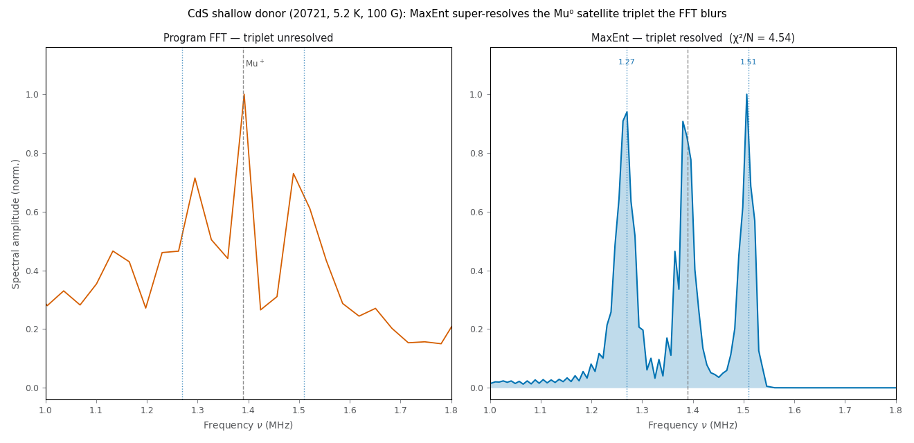
The base-temperature CdS run (20721, logged 5.175 K, 45.9 Mevents, TF 100 G). Left: the program FFT — at its native ≈ 32 kHz bin, no zero padding — renders the Mu⁰ satellite triplet as an unreadable comb of side-lobes about the central Mu⁺ line. Right: a MaxEnt reconstruction over a tight explicit window resolves three clean lobes at 1.27, 1.39, and 1.51 MHz — the central line and its two satellites. The measured satellite splitting, ≈ 0.214 MHz, is the shallow-muonium hyperfine constant. The reconstruction plateaus at χ²/N = 4.54 on this real forward/backward run, yet the lobe centres land on the expected positions.

The recipe is the tightly scoped one above, pushed to its limit:

• Set an explicit frequency window — 0.9–1.9 MHz here. Uncheck Auto window from field: at 100 G the field-derived window spans several MHz, so the reconstruction spends its amplitude budget on empty bins and blurs the very lines you are trying to separate.

• Bin the raw histogram (Binning ×4). Combining time bins shortens the design matrix and raises the counts per bin without touching the frequency resolution, which the window sets.

• Keep the spectrum grid compact — a 128-point grid across the narrow window is enough to separate lines 0.1 MHz apart. This is a genuine trade-off: too fine a grid lets the reconstruction ring, scattering spurious ripple between the lobes, while too coarse a grid merges them, so the compact grid is chosen deliberately rather than for speed.

• Run a modest number of cycles (about 20) and watch the Diagnostics line settle.

Note the honest caveat printed on the figure. On this real, high-statistics forward/backward run the χ² per degree of freedom plateaus near 4.5 rather than falling to 1 — the error model and background handling of a genuine run set a floor the entropy estimator cannot beat, and a plateau above 1 is expected on several real runs even where the reconstruction is visibly correct. The caution above therefore applies with full force: read the number and positions of the three lines, which are robust, and measure the splitting with a frequency-domain fit (Frequency-domain fitting) rather than off the lobe heights.

Reading the reconstruction overlay

The spectrum is what MaxEnt is for, but the time-domain reconstruction is how you check it. MaxEnt works by forward-modelling the raw counts: it asks what each detector group’s signal would look like if the data really came from the current spectrum, and adjusts the spectrum until those model signals match the measurements. The reconstruction overlay shows that comparison directly — the measured signal and the model the spectrum predicts, group by group, in time.

After a run, tick Show time-domain reconstruction in the MaxEnt panel. The plot workspace switches to a stacked view: one panel per detector group with the data and the reconstructed model on the same axes, and a residuals strip beneath showing the weighted residual \((d-m)/\sigma\). The χ² printed above the plot is the same number the Diagnostics line reports — it is computed from these very residuals, so the overlay and the convergence figure can never disagree.

Tick Combine groups on one axis to overlay every group’s data and model on a single colour-coded panel above one shared residuals strip, instead of the per-group stack. The combined view is the quicker read when you only want to see whether the whole fit holds together; the per-group stack is better for tracing left-over structure to a particular detector. Both report the same total χ².

This is the strongest single check of fit quality:

• A good fit sits on the data with residuals scattered evenly around zero and no left-over oscillation — the model has captured the precession.

• Left-over structure in the residuals (a coherent wiggle, a slow drift) means the spectrum is missing a line, has put it at the wrong frequency, or has the wrong phase for that group. Widen or re-centre the frequency window, re-seed the phases, and run again.

• Residuals that blow up at early or late times point at the time window or an instrumental artefact (deadtime at short times on a pulsed source; noise at long times) rather than at the spectrum itself.

The reconstruction is recomputed from the converged spectrum each run and is not stored in the project file; re-open the spectrum and run a cycle to regenerate it. Untick the box (or click the MaxEnt domain button) to return to the spectrum.

Pulsed sources: the pulse-shape response

At a pulsed source (ISIS) the muons arrive spread over a finite pulse of order tens of nanoseconds, so a precession signal that oscillates fast compared with the pulse is averaged across the spread of arrival times and its amplitude is suppressed. Above roughly 5 MHz this distorts the recovered spectrum: a real line at high frequency comes out with too little weight. Continuous sources (PSI, TRIUMF) do not have this limit, so the correction is off by default.

The Pulse shape controls fold the instrument response into the forward model, where it belongs — MaxEnt then reconstructs the true spectral weight rather than the attenuated one. Choose:

• Ignore — no pulse shaping (continuous-source data).

• Single pulse — one proton pulse of the given Half-width (μs).

• Double pulse — the ISIS double-pulse structure, with the Separation (μs) between the two pulses.

The response is a parabolic proton-pulse transform rolled off by the pion lifetime; the half-width and separation default to the ISIS values (about 50 ns and 0.324 μs) because the loaders do not yet record them per run. The effect is dramatic: on synthetic pulsed data with equal-amplitude lines at 1 and 7 MHz, the recovered 7 MHz weight is suppressed by a factor of ~4 with the response off and restored to roughly the 1 MHz weight with it on.

Excluding a time window

A laser flash, an RF burst, or a detector glitch can corrupt an interior stretch of the histogram. Set De-weight from / to (μs) to down-weight that window in the reconstruction. The points are de-weighted (their error bars are inflated so they carry essentially no weight), not removed, so the time grid — and any frequency resolution derived from it — is unchanged. This is why the control is named for de-weighting rather than exclusion (contrast the count fit’s hard Skip window; see Exclusions: a glossary of six mechanisms). Leave the fields blank to disable.

Field axis

A precession line at frequency ν corresponds to a local field B through ν = γ_μ B / 2π, with γ_μ/2π = 135.5 MHz/T. The spectrum’s X Units selector (above the plot) switches the axis between frequency (MHz) and field (Gauss or Tesla) without recomputing — handy when the science is a field distribution (a vortex lattice, an internal-field spread) rather than a frequency.

Shift axes

Next to X Units is an Axis: selector with three modes that transform the plotted spectrum itself (not just the axis labels):

• Absolute — the measured frequency/field, in the selected X Units.

• Shift (x − x₀) — each spectrum minus its reference field, shown in the selected unit (MHz, G, or T; the Larmor relation is linear, so a frequency shift is a field shift once unit-converted). The axis is labelled, for example, Field shift B − B₀ (G).

• Relative shift (ppm) — the dimensionless fractional shift (x − x₀)/x₀ × 10⁶, in parts per million (identical for frequency and field, so the X Units selector is inert here). The axis is labelled Relative shift (B − B₀)/B₀ (ppm).

The Ref.: selector (enabled in the shift modes) chooses the reference x₀:

• Run field (the default) — each spectrum uses its own applied field from the run/dataset metadata. This is the point of the feature: overlay several transverse-field runs measured at different applied fields and, in Shift (x − x₀), every line snaps to zero shift so a paramagnetic or Knight shift between them reads at a glance. A run with no field metadata is drawn untransformed (at its absolute position) and a note is logged, rather than dropped.

• Common — every spectrum shifts by the single value in the Gauss box, seeded from the active run’s field and freely overridable.

The reference field is not fitted here; the shift axes are a display transform for reading and overlaying spectra.

Calibration: phases, deadtime, and ZF/LF mode

MaxEnt needs one phase per detector group, and a good spectrum needs good phases. The Calibration controls connect MaxEnt to the rest of the analysis.

Phase exchange. If you have already fitted the run with a grouped time-domain fit, click Use fitted phases to seed the MaxEnt group phases from that fit (converted from radians to degrees). After MaxEnt has refined the phases, Send phases to fit writes them back to the grouped fit. A provenance line records which direction the exchange went and when. (Phases are matched by group id, so the forward/backward mapping never gets crossed.)

Note

The FFT per-group phases and the MaxEnt fitted-phase exchange are separate stores, by design. The Fourier panel’s per-group phase table (FFT Phase Modes, with its auto-estimate) and this MaxEnt exchange (which swaps phases with the grouped time-domain fit) hold the same physical quantity — the per-group detector phase — but do not feed each other: refining phases in MaxEnt does not update the FFT phase table, and filling FFT phase estimates does not seed MaxEnt. Keep them in sync by hand if you switch estimators on the same run. A “use MaxEnt fitted phases” pull on the Fourier panel is a plausible convenience and will be added on the first concrete request for it; until then the two stores are independent.

Deadtime. At a pulsed source the detectors lose counts at early times where the rate is highest, distorting the signal that carries the high-frequency information. Fit deadtime estimates a per-detector deadtime from the early-time count decay; Apply to grouping then promotes it to the run’s deadtime correction. The fit never changes the grouping on its own — you apply it explicitly, so the provenance is clear.

ZF/LF mode. In zero or longitudinal field the two detectors (forward and backward) measure the same relaxation with opposite phase. Select ZF / LF (two-group) as the mode: include exactly two groups, and MaxEnt pins their phases to 0° and 180° and ties their amplitudes through the run’s α (the detector-efficiency balance). The resulting spectrum is the field distribution p(B) — for a static Gaussian Kubo–Toyabe relaxation it is broad and centred near zero field rather than a sharp line. (The MaxEnt method is tuned more for transverse-field rotation than for zero-field precession, so read ZF spectra as distributions, not as resolved frequencies.)

Zero-frequency background (SpecBG). A ZF field distribution is dominated by its strong central peak, which can bury weak satellite structure. Enable Zero-frequency background (ZF/LF mode only) to subtract a zero-centred pseudo-Voigt model of that central peak from the displayed spectrum — the Gaussian and Lorentzian widths and the Lorentzian fraction shape the model. It is display-only and never alters the reconstructed spectrum.

Export. Export spectrum… writes the spectrum as text (frequency MHz, field G, density, with a parameter header); Export log… writes the per-cycle convergence trace and the final per-group phases, amplitudes, and backgrounds.

Choosing a spectral estimator: FFT, MaxEnt, or Burg

Asymmetry offers three ways to turn a time-domain signal into a spectrum, and they answer different questions. The first two are quantitative measurements; the third is a diagnostic.

Use the FFT for speed and linearity:

• The signal-to-noise ratio is good

• Fast, one-shot computation is what you need

• You want a linear transform that maps directly onto the standard apodisation knobs, with amplitudes and areas you can trust

Use MaxEnt for pulsed-source resolution and per-group phase handling:

• The data is noisy or the usable time window is short, and you need to pull a weak line out at higher effective resolution

• You are at a pulsed source and want the finite-pulse response folded into the forward model (see Pulsed sources: the pulse-shape response) rather than fighting the high-frequency rolloff afterwards

• You want one reconstruction that carries per-group phases and per-bin errors through to the spectrum (see Calibration: phases, deadtime, and ZF/LF mode)

• You are willing to drive the iterative refinement and watch it converge

Use Burg (the Resolution (Burg) display mode) only as a line-splitting diagnostic:

• You want to ask “is that one line or two?” — the all-poles estimate resolves close lines from a short window that collapse to a single FFT peak, and the pole count hints at how many components a fit should include

• You then read the count and rough positions and measure the lines with an FFT/MaxEnt spectrum or a frequency-domain fit — never off the Burg curve itself, whose peak heights are not amplitudes and which is prone to spurious splitting and noise-dependent position bias

The Burg method, its pole scan, and its pathologies are documented in Frequency-domain conditioning. Once you have a spectrum from any estimator, fit it quantitatively through Frequency-domain fitting.

The same line, two ways

The two quantitative estimators are most easily compared on one dataset. The figures below show the transverse-field signal of a YBCO vortex lattice — whose internal-field distribution \(P(B)\) is intrinsically asymmetric, with a sharp edge near the saddle-point field and a long tail towards the vortex cores — reconstructed both ways.

The FFT: a fast, linear transform of the (optionally apodised) asymmetry, framed on the precession line. The Fourier tab alongside holds the transform’s controls — the FFT phase mode, the Apodisation filter (shown at its None default), and Compute FFT.

The maximum-entropy reconstruction of the same run. Switch the frequency-domain workspace to MaxEnt and click Converge (or a +1 / +5 / +25 cycle button) on the MaxEnt tab alongside; the spectrum appears once the iteration converges.

Read on the same precession-frequency axis, the two are complementary: the FFT is immediate and its areas map onto the apodisation settings, while the MaxEnt reconstruction resolves the asymmetric line at higher effective resolution and carries the per-group phases, the per-bin errors, and — at a pulsed source — the pulse response through its forward model. Choose between them with the guidance above.

High-field FFT and MaxEnt on HAL data

The same comparison plays out on real high-field data. The organic antiferromagnet κ-(BEDT-TTF)₂Cu[N(CN)₂]Cl was measured in transverse fields of 6 and 8 T on the HAL9500 spectrometer at PSI [10]. At 6 T the diamagnetic Larmor line sits at 813 MHz (\(\gamma_\mu \cdot 6\,\text{T}\)), and the raw HAL .mdu histograms are binned finely enough — about 0.02 ns — that the transform reaches it directly, with no rotating reference frame. This is the corpus’s high-field frequency-domain example; the ordering transition and its order parameter are analysed as a temperature trend (Temperature scan through a magnetic transition) rather than repeated here.

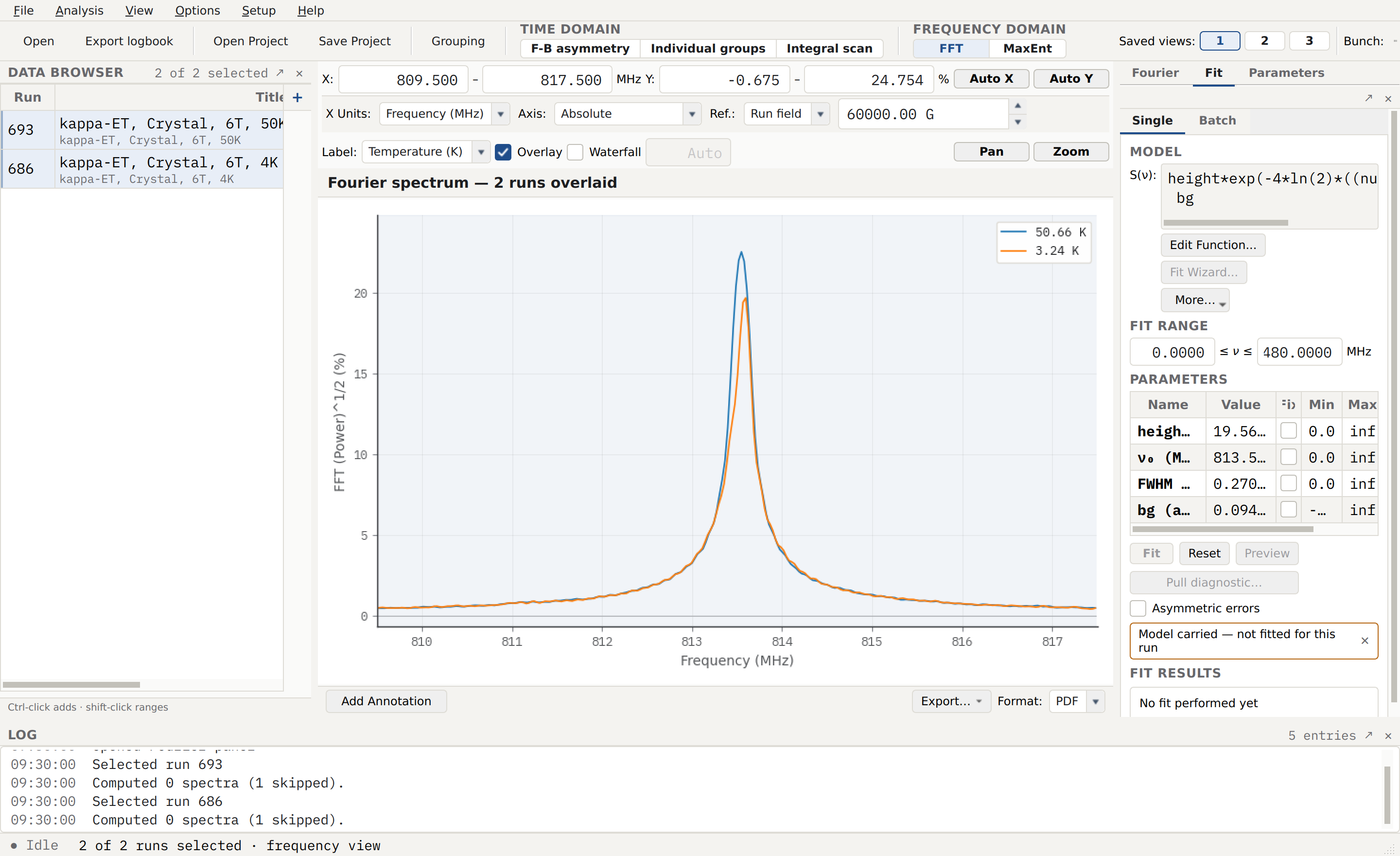
Two 6 T runs overlaid on the Frequency Domain tab through the GUI Fourier workflow multi-run overlay, with the plot’s Label combo set to Temperature (K) so the legend reads the temperatures directly. The paramagnetic run (50.66 K, above the transition) shows a sharp diamagnetic line at 813.5 MHz; the ordered run (3.24 K, below it) is visibly broadened and depleted — the antiferromagnetic order moves spectral weight out of the sharp central peak into the wings. The narrow 6 T line (~13 G wide at 813 MHz) is framed around its centre automatically, since on a from-zero axis it would be sub-pixel.

MaxEnt reconstructs the same line straight off the raw .mdu file. Its ≈ 389 000 time bins would make an unsteered reconstruction enormous, but with Auto workload steering (see Workload steering and the large-calculation warning) the engine sizes the settings you leave unset to the run — here raising Binning to 10 and capping the end time near 2 μs — and records what it chose in the result’s auto_steer_applied metadata.

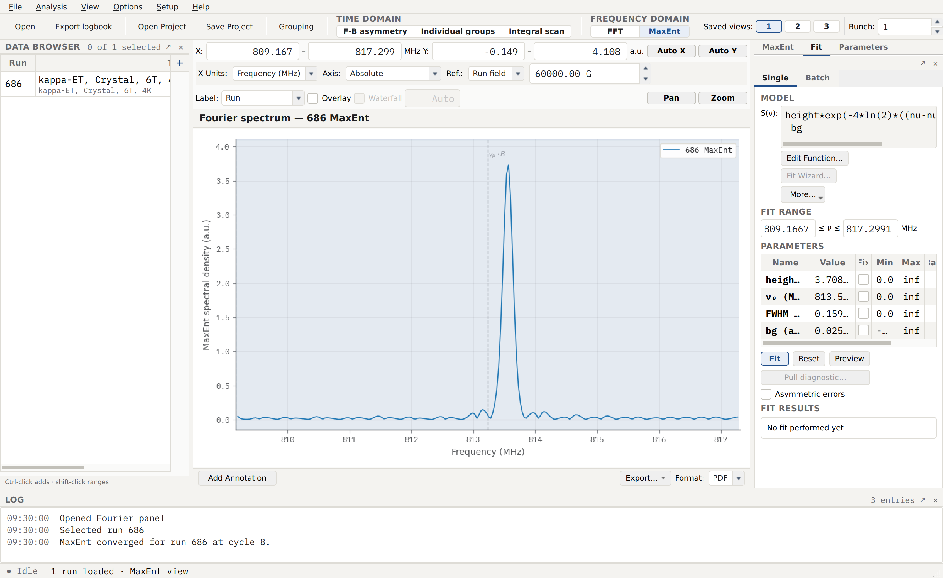
The base-temperature ordered run (686, 6 T, 3.24 K) reconstructed by MaxEnt from the raw HAL histograms with binning and end-time chosen automatically. The internal-field line lands at 813.56 MHz, just above the \(\gamma_\mu \cdot B\) applied-field marker at 813.3 MHz, and the calculation converges in eight cycles. The field-referenced ΔB axis the original study works in is one selector away through X Units and Axis: (Shift axes).

Practical example

Complete workflow for frequency analysis:

from asymmetry.core.io import load
from asymmetry.core.fourier.fft import fft_asymmetry
import matplotlib.pyplot as plt

# Load data
dataset = load("data.nxs")

   # Compute FFT with WiMDA-style Gaussian apodisation and 4× zero-padding
freq, real_part, magnitude = fft_asymmetry(
    dataset,
      window="gaussian",
      filter_start_us=0.2,
      filter_time_constant_us=1.5,
    padding_factor=4,
    t_min=0.1,
    t_max=10.0,
)

# Plot
fig, (ax1, ax2) = plt.subplots(2, 1, figsize=(10, 8))

# Time domain
ax1.errorbar(dataset.time, dataset.asymmetry, yerr=dataset.error, fmt='.')
ax1.set_xlabel("Time (μs)")
ax1.set_ylabel("Asymmetry")
ax1.set_title("Time Domain")

# Frequency domain
ax2.plot(freq, magnitude)
ax2.set_xlabel(r"$\\nu$ (MHz)")
ax2.set_ylabel(r"$|\\mathcal{F}|$")
ax2.set_title("Frequency Domain (FFT with Gaussian apodisation)")
ax2.set_xlim(0, 50)  # Focus on 0–50 MHz

plt.tight_layout()
plt.show()

GUI Fourier workflow

The FFT spectrum computes automatically the moment you look at it. Opening the Frequency Domain tab — via the plot workspace’s tab strip or the toolbar FFT button — for a run that has never been transformed synthesises a recipe from the current Fourier panel settings and the run’s own detector grouping, then runs the transform off-thread behind a busy overlay (“Computing FFT for run <n>…”) so the window stays responsive. Switching to a different run while the Frequency-domain tab is showing does the same: each never-computed run picks up a fresh spectrum as you select it. Compute FFT, pinned in the action footer at the bottom of the Fourier panel (always visible, outside the scrolling settings area), remains the explicit way to re-run the transform after you change a setting — auto-compute only ever fills a genuinely empty spectrum, it never overwrites one you have already computed. The button acts on the full Data-Browser selection and its label counts the scope (see Computing for a selection).

A multi-run overlay extends the same idea to a selection: toggling Overlay with several runs selected auto-computes every member that has no spectrum yet, in waves of 25 runs at a time (an overlay status of “Computing FFT for <n> run(s)…”), re-rendering after each wave until every selected run is included. Runs that cannot compute — no detector groups, or a transform that fails — are skipped and reported in the status line: “Overlaying <n> runs; <m> selected run(s) could not be computed — check their detector grouping and the log.”

The overlay’s legend takes its labels from the plot panel’s own Label: combo — the same metadata-field picker the time-domain view uses — so a run number, field, temperature, or comment identifies each trace. Choosing Temperature (K), for example, renders each entry as its value alone (for example 3.24 K), which is the natural way to compare, say, an ordered run against a paramagnetic one and read the line broadening between them directly off the legend.

Once several spectra are overlaid, Waterfall stacks each one onto its own vertical offset so nearby lines stay resolved instead of overlapping — see waterfall stacking for the shared control (it works the same way here as on the time-domain panel, except that a spectrum’s own baseline stands in for the time-domain hairline).

The first view is also framed to where the physics is. A narrow line at high frequency — a 6 T Larmor line is ~13 G wide at 813 MHz — is framed around (the line centred, the window a few dozen linewidths wide: WiMDA’s reference-field ± offsets view, derived from the data), because on a from-zero axis it would be sub-pixel. Otherwise the plot frames from the data’s lower edge up to the highest-frequency line that clears the local noise baseline, and — when the run carries an applied field — at least the expected Larmor region γ_μ·B. The widest need wins: a second real line (AFM satellites, muonium triplet lines, muoniated-radical pairs) is never framed out, and a weak or low-field line that the peak detection cannot see still gets a sensible window instead of the full Nyquist span. Spectra also default to a zero-pad factor of 4, so line shapes arrive sinc-interpolated rather than 2–3 bins wide; this deliberately diverges from WiMDA’s no-padding default because the spectrum is now shown unbidden, and it changes nothing quantitative — zero padding adds no information, only smoother rendering. Padded points are strongly correlated (only 1/n of them are statistically independent for a zero-pad factor n), so frequency-domain fits and moment uncertainties apply the effective-sample-size correction automatically: degrees of freedom count the independent samples, χ² is scaled to match, and parameter/moment uncertainties grow by √*n*. Fit results state the applied correction in their advisory row. (WiMDA applies the degrees-of-freedom part of this correction — dof := n div zpad — Asymmetry additionally corrects χ² and the uncertainties for full consistency.) With the statistics handled, the zero-pad factor is purely a display-density knob; the factor now goes up to 64. All of these are first-paint seeds only: your own zoom and settings are never overridden.

Auto-compute needs detector groups to work from. A run with no groups (or with every group excluded), or one whose transform genuinely fails, cannot seed a recipe and instead shows a centred prompt over the Frequency-domain plot — “No FFT spectrum for this run. Spectra compute automatically when the run has detector groups — check the grouping and the log, or click Compute FFT to retry.” — instead of a blank tab. That prompt is the “cannot auto-compute” state, not a broken transform, and it clears the moment a spectrum is computed.

To see an FFT spectrum:

1. Select the run in the Data Browser. Selecting a run populates the Fourier panel’s Groups table (Group 1 / Group 2 …). With no run selected the Groups table — and therefore the spectrum — stays empty.

2. Open the FFT view — the toolbar FFT button raises the Fourier panel and switches the central plot to the Frequency Domain tab. If the run has never been transformed, the spectrum computes automatically at this point (behind the busy overlay); if it already has one, that spectrum is shown directly.

3. (Optional) Tune the settings — phase mode, apodisation, included groups, phases — using the controls described below.

4. Click Compute FFT in the panel’s pinned action footer to apply any settings you changed. Auto-compute only fills a never-computed run, so this click is still how you re-run the transform with new parameters.

While the Frequency-domain tab has no spectrum and cannot auto-compute one, the plot shows the empty-state prompt above and the status line reads No FFT computed for run <n> — check the run’s detector grouping (and the log for a failed transform), or click Compute FFT to retry.

Before you click Compute FFT, the docked Fourier panel lets you tune the WiMDA-first FFT workflow directly:

• choose an FFT Phase Mode first. The Info button beside it opens an in-app explanation of the formulas and interpretation of each mode

• keep Subtract average signal enabled to remove the WiMDA-style pre-FFT baseline term before filtering and transformation; this is on by default

• grouped Fourier inputs are also corrected for the muon decay envelope before the later mean-subtraction and apodisation steps, matching WiMDA’s grouped Freq preprocessing more closely

• choose None, Lorentzian, or Gaussian apodisation, then tune the filter start and tau values to match WiMDA-style FFT shaping

• include or exclude detector groups in the Groups table before computing the transform

• in Phase mode, either type a single manual phase or enable Use per-group phase table and edit the per-group values

• choose Auto method (Peak or Average), then press Fill Phase Estimates to estimate one phase per detector group for the current dataset

• for averaged grouped spectra, optionally estimate WiMDA-style error bars from the spread across the selected group spectra

Out-of-date indicator

A computed spectrum stays on screen when you keep working, so the panel tells you when the display no longer matches the current settings. Editing any FFT parameter, or changing the time-domain fit range the transform inherits, raises an amber banner directly above the action footer:

Spectrum out of date — <what changed>. Compute FFT to refresh.

The banner names what changed (for example zero-pad factor, apodisation changed) and clears on the next Compute FFT. Nothing recomputes automatically for these two triggers — the displayed spectrum is never replaced behind your back — and parameters that are inert in the active mode never flag: a filter τ edit while apodisation is None does not mark the spectrum out of date, and a time-range change already absorbed by the good-statistics tail cap does not either.

Applying a new grouping — or a t0, deadtime, or background change through the grouping dialog — is handled differently: the FFT spectrum “follows the data” the same way the time-domain plot does. A spectrum computed under the old grouping is not merely stale, it is wrong, so applying a regroup discards the affected runs’ FFT spectra and recipes outright (logged as “Discarded <n> FFT spectrum(s) computed under the previous grouping; they recompute on next view.”) and, if the Frequency-domain tab is the active view, recomputes it immediately rather than leaving the stale banner up. There is nothing to refresh by hand here — the next view of the run gets a fresh spectrum against the new grouping automatically.

Computing for a selection

Compute FFT is selection-scoped: it computes every run selected in the Data Browser, or the active run alone when nothing else is selected. The button’s label shows that scope before you click — Compute FFT for a single run, Compute FFT (3 runs) when three runs are in scope — and its tooltip reads:

Compute FFTs for every run selected in the Data Browser using the current settings. The Groups table’s enabled groups apply to every run; phases stay per-run.

Every run in scope is recomputed from the CURRENT panel state — apodisation, padding, display mode, phase mode, and conditioning. The Groups table’s enabled groups apply to every run in the selection, intersected with each run’s own available groups — a series computes with one consistent group inclusion, and each target’s stored Groups table is updated to match, so visiting it later shows the propagated inclusion, in sync with its spectrum. Phases stay per-run: each run’s phase values come from its own stored phase table (or defaults). A run whose groups have no overlap with the enabled set — or that has no detector groups at all — is skipped and reported in the status line (“Computed <n> spectra (<m> skipped).” — the skipped count appears only when runs were skipped). The implicit compute-on-view fill and the overlay auto-compute are unchanged: they keep each run’s own stored inclusion; only the explicit button propagates the panel’s. Computation runs off the GUI thread, and on completion the central workspace switches to the Frequency-domain view and renders the result — the active run’s spectrum, or the full overlay when the Overlay toggle is on with several runs selected.

This consolidation replaces an earlier Apply to selection affordance that copied the active run’s already-computed recipe onto the other selected runs without reading the live panel state, so a setting changed after the last Compute FFT was silently left out, and did not re-render the view. That compute-once-copy-around model is gone: Compute FFT always reads the panel as it stands now and always acts on the scope its label names.

Because overlay members can be computed independently — one earlier under different settings, one auto-filled by the overlay itself — they can drift out of alignment with each other. When an active overlay mixes spectra computed under different settings, the panel raises a second banner, independent of the out-of-date indicator below:

Overlaid spectra use different settings — Compute FFT to unify.

The comparison is cheap (stored recipe dictionaries only, no recomputation) and only looks at the runs actually in the overlay; a Compute FFT with the mismatched runs selected recomputes them all under one configuration and clears the banner.

Fitting the displayed spectrum

Once a Fourier spectrum has been computed, the Frequency workspace can be fit through the same Fit dock used for time-domain analysis. The fit target is the displayed real-valued spectrum. V1 provides Gaussian and Lorentzian peak components with constant or linear backgrounds; successful global frequency fits send nu0 and fwhm values, plus derived B0 and Bwid field equivalents, to the Parameters dock for trend analysis. See Frequency-domain fitting for the full workflow.

A single-run fit needs a single spectrum, so fitting is blocked while an overlay is active: the Fit dock disables and reports “Multiple spectra overlaid — select a single run to fit in the frequency domain.” Untick Overlay (or select just one run) to fit again.

Phase estimation workflow

Phase estimation in the GUI is explicit rather than always-on:

• estimates are only generated when you press Fill Phase Estimates

• the selected Auto method determines how the single-group FFT phase is measured within the current phase-estimation window

• when a field value is available, that window is narrowed around the expected precession frequency; otherwise the positive-frequency FFT range is used

• the estimated values are written into the per-group phase table for the current dataset only

The phase colour cues in the table are also meaningful:

• blue: the phase value is currently active and will be used

• grey: the phase value is present but not currently active

• green: the phase value was auto-estimated for the current dataset via Fill Phase Estimates

Asymmetry makes two explicit design decisions for this workflow, in the default Grouped average Signal source:

• Fourier transforms use grouped detector-count signals rather than the FB asymmetry trace as the input source. (The F−B asymmetry signal source is the deliberate exception — see Signal source.)

• The frequency-domain plot shows the average of the currently included groups rather than separate per-group spectra.

The FFT therefore uses the current grouped/bunched data definition. The grouped detector-count signal is rebuilt with the current bunching factor before the transform, and that grouped count signal is lifetime-corrected before the later subtract-average and filter stages. The FFT bandwidth and frequency spacing therefore track the effective binned timestep in the same way they do in WiMDA.

The Fourier panel is scrollable so these controls remain usable when the dock is narrow.

Frequency-domain plot behaviour

FFT output is shown on the dedicated Frequency Domain tab in the central plot workspace. Spectra draw as solid lines — the convention of every reference muSR package — with a shaded ±1σ band when the spectrum carries per-point errors (enable Average errors to compute them), rather than the time domain’s error-bar points. When the run’s applied field is known, a subtle dashed marker sits at the expected Larmor position γ_μ·B on the single-run view, answering “am I looking at the right place?” at a glance; it is omitted on multi-run overlays and the correlation axis, and it never appears in GLE/PDF exports (those draw from the data, not the screen). Each loaded run keeps its own frequency-domain view state in the session. Opening that tab for a run that has never been transformed computes its spectrum automatically (see GUI Fourier workflow); a run whose spectrum cannot be auto-computed — no detector groups, or a failed transform — shows the centred empty-state prompt on that tab instead — “No FFT spectrum for this run. Spectra compute automatically when the run has detector groups — check the grouping and the log, or click Compute FFT to retry.” Entering the Frequency-domain view stays on that tab whether it is computing, showing a spectrum, or showing the prompt; it no longer silently falls back to the time view, so the cue is always where you are looking. The current x-range is preserved across the switch. (The MaxEnt spectrum tab is unchanged: it is compute-on-demand, with its own “No MaxEnt spectrum computed…” prompt.)

The frequency viewer stores canonical FFT x-data in absolute MHz; the X Units and Axis: selectors above the plot choose how it is displayed (absolute, shift, or ppm — see Shift axes above). In the shift modes the plot, the tick labels, and the x-limit boxes all share one reference-shifted scale.

Exporting the spectrum

The plot toolbar’s Export… menu offers Export to GLE… (a compiled figure with editable .gle script and data sidecars) and Export plotted data (text)… (the sidecar files alone). On the frequency tab both mirror what is on screen rather than the time-domain idiom:

• Display units and window. The x column and the exported axis window are written in the current display mode — MHz, Field (G/T), a shift (shift_G…), or relative_shift_ppm — matching the on-screen axis. Real axis titles (for example Field shift B − B₀ (G) and FFT Magnitude (a.u.)) replace the time-domain labels.

• Line and band. A spectrum draws as a solid piecewise-linear line plus a light shaded ±1σ band behind it, matching the screen (GLE has no fill transparency, so the band compiles as a light tint of the series colour); the band is omitted when the spectrum carries no per-point errors.

• Self-describing sidecars. Each .dat names its columns in the header (for example shift_G  amplitude  error  frequency_MHz) and keeps the canonical frequency_MHz axis as a trailing column whenever the display differs from absolute MHz — including every shift/ppm export — so the raw spectrum is always recoverable. A START OF FOURIER INFORMATION block records the display mode, apodisation and zero-pad settings, the axis mode, and each spectrum’s own reference field.

References

[1]

10. 23. Cooley and J. W. Tukey, Math. Comput. 19, 297 (1965).

[2] (1,2)

10. Skilling and R. K. Bryan, Mon. Not. R. Astron. Soc. 211, 111 (1984).

[3]

2. 4. Rainford and G. J. Daniell, Hyperfine Interact. 87, 1129 (1994).

[4]

6. 12. Pratt, Physica B 289–290, 710 (2000).

[5]

20. 13. Riseman and E. M. Forgan, Physica B 289–290, 718 (2000).

[6] (1,2)

S. J. Blundell, R. De Renzi, T. Lancaster, and F. L. Pratt, Muon Spectroscopy: An Introduction (Oxford University Press, Oxford, 2022), §15.5.

[7]

6. 10. Harris, Proc. IEEE 66, 51 (1978).

[8]

10. 13. Gil et al., Phys. Rev. Lett. 83, 5294 (1999).

[9]

10. 13. Gil et al., Phys. Rev. B 64, 075205 (2001).

[10]

B. M. Huddart, T. Lancaster, S. J. Blundell, Z. Guguchia, H. Taniguchi, S. J. Clark, and F. L. Pratt, Phys. Rev. Research 5, 013015 (2023).

The phaseOptReal entropy phase optimiser reproduces the PFTPhaseCorrection routine of musrfit (A. Suter and B. M. Wojek, Phys. Procedia 30, 69 (2012)).