Joint fits
Each ordinary time-asymmetry series retains its canonical model’s fixed time response in joint fitting and replay. Shared parameter columns do not estimate pulse separation.
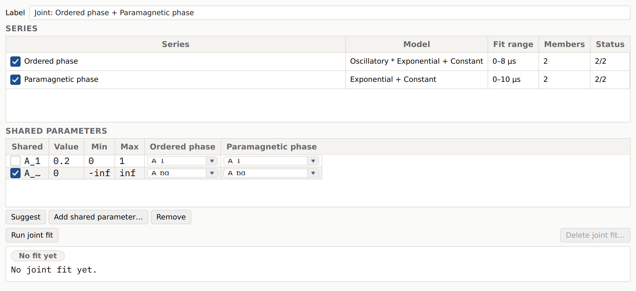
The joint-fit window on a sample crossing a phase transition: an ordered
phase fitted with Oscillatory * Exponential + Constant and a
paramagnetic phase fitted with Exponential + Constant, both ticked.
“Suggest” has proposed the background A_bg as an exact, ticked match
and the amplitude A_1 as an unticked candidate — the two models expose
their own amplitude as one parameter each, but that alone does not make the
quantities the same, so the tiering leaves the decision to the user.
When to use a joint fit
A sample measured across a phase transition often needs two different fit functions: an oscillating model in the magnetically ordered phase and a relaxing model in the paramagnetic phase above it. Some quantities are the same physical thing in both regimes — the initial asymmetry, the background, alpha, an instrumental phase — and a fit that ignores this measures them twice, independently, and then hopes the two answers agree.
Until now the only way to share a parameter was the Batch tab’s Global role, which shares a parameter across the runs of one series fitted with one model (see Global fitting in Fitting engine). Two series with different models could not share anything: you fitted them separately and compared the numbers afterwards. A joint fit puts both series into one cost function, with one column for the shared quantity, so its value is estimated from every run of both series at once and its uncertainty propagates correctly into everything else.
A joint fit does not replace the Global role, and it does not let you build
a new model. It composes series you have already made: each member is an
ordinary FitSeries — its
model, its member runs, its fit range, its parameter table — exactly as
recorded from the Batch tab. The joint fit adds only a table of shared
parameters and its own label. If you need to change a member’s model, seeds,
bounds, or fit range, edit that series on the Batch tab as you always would;
the joint-fit window itself edits no recipe.
The three scopes
Asymmetry now has three, deliberately distinct, notions of “one value shared across several things”:
Local — one fitted value per run. The Batch tab’s default classification for every parameter.
Global — one fitted value per series, shared across every run that series covers. Set in the Batch tab’s parameter table; unchanged by anything below.
Shared — one fitted value across two or more series, set up in the joint-fit window. A shared parameter must be a Global parameter of every series that contributes to it — Local and Fixed rows are never offered, because they do not denote “one value for this series” in the first place.
Two older words keep their existing meanings and are not reused here. “Linked” still means the Batch/Single tab’s equality link groups (the ⇄ badge) — a per-series device that ties two parameters of the same run’s fit together. “Global Parameter Fit” still names the separate cross-group analysis window (GUI usage’s Global parameter fit window) that fits a trend parameter such as λ(B) across several data groups. Neither is a joint fit, and a joint fit does not change what either of them does.
Setting up a joint fit
Open Analysis ▸ New joint fit… for an empty window on the active representation, or pick a recorded one from the Analysis ▸ Joint fits submenu (a stale entry is suffixed “ (stale)”; see Staleness and detaching below).
The Series section lists every series of the active representation, with its model, its Fit range, its member count and its status (how many members converged when it was last fitted, and at what time). Each member is fitted over its own range — the one set on the Batch tab when the series was recorded — so two members may cover different windows; a series recorded without a range reads “Plot’s fit range” and uses the range set on the plot. Change a member’s range on the Batch tab. Only a time-domain, run-membered series with a fit model can be a member; everything else is listed disabled, with the reason on its tooltip:
a detector-group series reads “Detector-group series”,
a model-less (computed) series reads “No fit model”,
a series that shares a run with one already ticked reads “Shares runs with <other series>” — a run may belong to exactly one member, so the window prevents the overlap by disabling the conflicting row rather than letting you create a cost function that would weigh the same data twice.
A frequency-domain representation offers no series at all: “Joint fits are available for time-domain series only” (a zero-padded Fourier spectrum’s samples are correlated in a way the joint solver does not yet account for).
Tick two or more eligible series. The Shared parameters table then grows one column per ticked series, alongside Shared, Value, Min, and Max:
Suggest proposes rows from the ticked series’ models and their Global parameters, in two tiers:
an exact row — the same full parameter name, the same unit, appearing exactly once in every model, and Global in every series — is ticked by default;
a candidate row — the same base name at a different component index (
A_1here,A_2there), or the same base name owned by a different component type in each model — is proposed unticked, for you to judge.
A row you have added by hand, or edited, survives a re-run of Suggest; only an untouched, machine-proposed row is replaced.
Add shared parameter… prompts for a name and adds an empty row you fill in yourself: tick a Global parameter for each contributing series from its column’s dropdown (the dropdown’s placeholder entry, “—”, means “this series does not contribute this row”).
Remove drops the selected row(s).
A shared row’s seed and bounds come from the first ticked series that contributes to it (in tick order) — never averaged across contributors, since the shared value is a new fitted quantity and averaging two series’ own seeds would invent a number neither of them holds. Edit the Value, Min, or Max cell directly to override. Every other seed, bound, fixed or file-pinned value, and the fit range, is read from each member’s own recipe exactly as a solo Batch-tab run of that series would read it — the Batch tab’s inherited single-fit seeds and its Initial-values dialog do not apply here. Each member’s fitted curve is drawn over that same fit range, so a series whose range starts at 0 has its curve reach back to t = 0 even when the first data point sits later.
The initial-asymmetry caveat. “Initial asymmetry” is shareable only when
a model exposes it as one parameter — a fraction group with one overall amplitude budget across its additive
terms is exactly this case. A model
that instead sums several independent component amplitudes has no single
column that is the initial asymmetry; constraining that sum to a shared
value is a genuine physical constraint, but it is not what a shared
parameter expresses, and v1 does not offer it. This is why the suggestion
above proposes A_1 only as a candidate: the same name can be the sole
amplitude of one model and one term among several in another.
The Label field defaults to “Joint: <series> + <series>”, built from
each ticked series’ short name — its own label, else its data group’s
name, else its model’s expression — rather than that series’ full
<model> · <fit-range>[ · <group>] fallback name, which is what made an
early build’s default read as “Joint: OverhauserPowderCutoff ·
0.002–0.1 µs · low + Exponential · 0.002–0.1 µs · high”. Two ticked series
that still resolve to the same short name (no label, no group, the same
model) fall back to that series’ full name so the label stays unambiguous.
The field’s tooltip always lists every ticked series’ full name, one per
line, so the full picture is one hover away even when the label itself is
short. Type in the field to set your own label, which then survives further
re-runs and re-suggestions.
Click Run joint fit to fit. Stop cancels a running fit and leaves every member’s previous results exactly as they were — nothing is recorded for a fit that did not finish, or did not converge.
Results
A converged joint fit writes its results onto the member series themselves, in place, under their existing recording — a joint run does not create a new series, because the recipes did not change, only the constraint on them. Each member’s per-run results carry the shared value under that series’ own parameter name, so every existing consumer (the Fit Parameters panel, an export, the plot overlay) reads a jointly fitted series exactly like any other.
The results card shows the combined χ²ᵣ and degrees of freedom, each shared parameter’s fitted value and uncertainty, and one row per member series with its own χ²ᵣ (computed as if that series had been fitted alone) and an Open in Batch tab button.
The Fit Parameters panel groups a joint fit’s member series into their own chip-rail section, titled with the joint fit’s label, ahead of the ordinary data-group sections — a joint fit can span series that belong to different groups or carry different models, so its own section is what shows “these belong to one coupled fit” without you having to infer it from a badge alone. The section header’s tooltip lists every member’s full name, one per line.
A shared parameter is, in every contributing series, still a Global one, and “Global” means one value per series everywhere in the app: it gets no chip, no card, and is never plotted as a per-run trend, exactly like any other Global parameter. The footer’s existing note (”<name> Global — held constant”) names it too, and for a shared parameter that note’s entry gains a suffix naming the joint fit it is shared across: “<name> — shared across joint fit “<label>””. Joining a joint fit does not change a parameter’s Global-role behaviour; it only adds that one extra clause to the hint for the column the joint fit actually shares. See Joint-fit series in Parameter trending for the full anatomy of the chip-rail section and the hint.
Staleness and detaching
A joint fit’s staleness is never stored — it is computed from the live project every time you open the window, and shown as a banner across the top (“This joint fit is out of date: <reason>.”) with a Refit button that re-reads the current series and re-runs. The reason is one of:
“member series ‘<name>’ was deleted” — a member no longer exists;
“member series ‘<name>’ was re-run on its own” — someone re-ran that series from the Batch tab, which always detaches it: a solo Batch-tab run is never blocked by, and never honours, a joint fit’s constraint, so its fresh results no longer agree with the shared value the record holds;
“member series ‘<name>’ is stale (its membership changed)” — the member itself is stale against its own data group, independent of the joint fit.
The Batch tab is never blocked by a series’ joint-fit membership: re-running a member on its own is always allowed, and simply marks the owning joint fit stale rather than being refused.
Deleting
Delete joint fit…, confirmed with “Delete the joint fit ‘<label>’? Its member series and their results are kept; only the joint fit and its shared-parameter table are removed.”, removes only the record — every member’s results stay exactly as fitted. Deleting a member series instead (from its chip menu’s Delete series…, as for any series) removes it from the joint fit; a joint fit left with fewer than two members is deleted along with it, since a joint fit of one series composes nothing.
Scripting
The GUI sits on asymmetry.core.fitting.joint.fit_joint(), which takes one
JointSeriesProblem per series (its
datasets, model function, global/local parameter names, and one
ParameterSet of seeds per run) and a list of
SharedParameter rows naming, for each
series, which of that series’ Global parameters the row maps to:
import numpy as np
from asymmetry.core.fitting import (
    JointSeriesProblem, SharedParameter, Parameter, ParameterSet, fit_joint,
)

def oscillating(t, A, freq, Lambda, A_bg):
    return A * np.cos(2.0 * np.pi * freq * t) * np.exp(-Lambda * t) + A_bg

def relaxing(t, A, Lambda, A_bg):
    return A * np.exp(-Lambda * t) + A_bg

ordered = JointSeriesProblem(
    key="ordered",
    datasets=ordered_datasets,          # runs 101, 102 — ordered phase
    model_fn=oscillating,
    global_params=["A", "A_bg"],
    local_params=["freq", "Lambda"],
    initial_params={
        101: ParameterSet([
            Parameter("A", 16.0, min=0.0), Parameter("A_bg", 0.0),
            Parameter("freq", 1.1, min=0.0), Parameter("Lambda", 0.4, min=0.0),
        ]),
        102: ParameterSet([
            Parameter("A", 16.0, min=0.0), Parameter("A_bg", 0.0),
            Parameter("freq", 1.4, min=0.0), Parameter("Lambda", 0.4, min=0.0),
        ]),
    },
)
paramagnetic = JointSeriesProblem(
    key="paramagnetic",
    datasets=paramagnetic_datasets,      # runs 201, 202 — paramagnetic phase
    model_fn=relaxing,
    global_params=["A", "A_bg"],
    local_params=["Lambda"],
    initial_params={
        201: ParameterSet([
            Parameter("A", 13.0, min=0.0), Parameter("A_bg", 0.0),
            Parameter("Lambda", 0.4, min=0.0),
        ]),
        202: ParameterSet([
            Parameter("A", 13.0, min=0.0), Parameter("A_bg", 0.0),
            Parameter("Lambda", 0.4, min=0.0),
        ]),
    },
)

shared_background = SharedParameter(
    name="A_bg_shared",
    members={"ordered": "A_bg", "paramagnetic": "A_bg"},
    value=0.0,
)

result = fit_joint([ordered, paramagnetic], [shared_background])

print(result.shared_parameters["A_bg_shared"].value,
      "±", result.shared_uncertainties["A_bg_shared"])
print(result.reduced_chi_squared)
for key, chi2r in result.series_reduced_chi_squared.items():
    print(key, chi2r)
Every run of every member carries the shared value, and its one shared
uncertainty, under that series’ own parameter name in
result.series_results[key][run_number] — a downstream consumer that only
knows about ordinary FitResult objects needs
to know nothing about joint fitting to read a jointly fitted run.
asymmetry.core.fitting.joint.suggest_shared_parameters() is the autodetection
behind the window’s Suggest button: pass it the member models (in series
order) and, for each, a {parameter name: role} mapping, and it returns a
list of SharedSuggestion, each with a
tier of "exact" or "candidate" and a one-line rationale:
from asymmetry.core.fitting import CompositeModel, suggest_shared_parameters

ordered_model = CompositeModel.from_expression("Oscillatory * Exponential + Constant")
paramagnetic_model = CompositeModel.from_expression("Exponential + Constant")

suggestions = suggest_shared_parameters(
    [ordered_model, paramagnetic_model],
    [
        {"A_1": "global", "frequency": "local", "phase": "local",
         "Lambda": "local", "A_bg": "global"},
        {"A_1": "global", "Lambda": "local", "A_bg": "global"},
    ],
)
for s in suggestions:
    print(s.name, s.tier, s.rationale)
# A_1 candidate  A_1 appears once in every model, but on different components
#                (Exponential, Oscillatory).
# A_bg exact     A_bg appears once in every model with the same unit and the
#                Global role.
fit_joint raises rather than silently doing something else with a
malformed request: fewer than two series, a run number present in two
series, a shared row naming fewer than two members, a member that is not a
Global parameter of its series, a member a series pins on every run, the
same parameter shared twice, or strategy="profiled".
Limits in this version
Time-domain series only. The status line the window shows for a frequency-domain representation is exactly “Joint fits are available for time-domain series only” (see Setting up a joint fit above).
Run-membered series only. A detector-group (
member_kind ==
"groups"
) series cannot be a member; count-domain grouped fitting is not part of a joint fit in this version.Series-Global parameters only. A shared column always maps to a Global role in every contributing series; you cannot share a Local (per-run) parameter across series.
Equality only. A shared parameter is held exactly equal across its members; there is no affine or expression relation (no “twice this other series’ value”) across series. Within one series, ordinary equality link groups still work exactly as before.
Sparse least-squares solver.
fit_jointreports Gauss–Newton(JᵀJ)⁻¹uncertainties from a bounded sparse trust-region solve (or, withstrategy="joint", one Minuit HESSE covariance over the whole vector). There is no MINOS support for a joint fit, andstrategy="profiled"raises: it profiles one shared set of globals over datasets that already share one model, which a joint fit’s differently modelled series do not.No wizard entry point yet. The Global Fit Wizard’s phase partition does not yet offer “make these phases a joint fit” — for now, record each phase’s series from the wizard or the Batch tab as usual, then compose them from Analysis ▸ New joint fit….