Integral scan mode (avoided-level-crossing field scans)
The Integral scan mode turns a set of runs taken at different fields (or temperatures) into a single field scan: one integral-asymmetry value per run, plotted against the swept variable. It is the workflow for avoided level crossing (ALC), repolarisation / decoupling, and quadrupolar level-crossing resonance (QLCR) measurements, where a resonance appears as a dip or step in the asymmetry as the field is stepped through the crossing. The technique is often called an ALC scan, and the mode is labelled Integral scan (ALC) in the interface.
Unlike the time-domain fitting workflows, the Integral scan mode does not
fit a model to each spectrum. It reduces every run to one number — the asymmetry integrated
over a time window — and then lets you fit a baseline and resonance peaks to the
resulting scan. The method follows WiMDA’s count-integral ALC and Mantid’s
PlotAsymmetryByLogValue; with \(\alpha = 1\) it reproduces the WiMDA
count integral exactly.
The integral-asymmetry observable
For each run, the forward and backward counts are summed over the integration window \([t_\mathrm{min}, t_\mathrm{max}]\) and combined into a single asymmetry value:
where the sums run over the good bins inside the window, \(F\) and \(B\) are the forward and backward grouped counts, and \(\alpha\) is the current calibration constant from your detector grouping. Summing the counts before forming the ratio (the WiMDA “count integral”) gives Poisson-weighted statistics across the whole window rather than averaging per-bin asymmetries.
Each value is plotted against the run’s swept variable to form the scan. A resonance shifts the time-averaged asymmetry, so it shows up directly as a feature in \(A\) versus field. The dA/dB view (see below) plots the field-derivative of the scan — WiMDA’s differential ALC — which sharpens a resonance into a peak–trough signature.
Entering the Integral scan representation
ALC mode is the Integral scan representation, a button in the Time domain cluster of the main toolbar (alongside F-B asymmetry and Individual groups). Click it to enter — no separate toggle. It is always available; the two-or-more-runs requirement is checked when you build the scan, not when you select the representation.
When it is active:
the central plot area shows the field scan itself (the ALC curve), with a slim integration-window strip beneath it (see the integration window below);
the Fit dock shows the Integral scan (ALC) build panel — the Integration window spinboxes, the RF resonance option, and the Build Scan button;
the Parameters dock shows the scan’s analysis controls — the Baseline, Peaks, and RF resonance sections.
This is the key change from earlier versions: the scan is the main window, not a panel tucked into a dock. In scan mode you no longer interact with the per-run time spectra — they are only integrated — so the scan occupies the centre and the analysis controls stay to the side.
Switching to another representation keeps your scan and its analysis; they reappear when you return to Integral scan.
The ALC workflow
Step 1 — Build the scan
Load and multi-select the runs. Load the field-scan runs, then select them all in the Data Browser: click the first row and Shift-click the last (the scan is built from the current selection, exactly like a batch fit). The Data Browser resolves the B (G) column from each run’s field; that column becomes the scan’s field axis.
Select the Integral scan representation. Click Integral scan in the toolbar’s Time-domain cluster. The central area switches to the scan view (empty until you build), and the Fit dock shows the build panel.
Set the integration window. The window is the time-spectrum fit range. Drag the shaded window on the integration-window strip below the scan, or type precise \(t_\mathrm{min}\) and \(t_\mathrm{max}\) values (in μs) into the spinboxes in the Integration window group of the build panel. The strip, the spinboxes, and the F-B time plot all stay in sync.
Press Build Scan.
Each selected run is integrated over the window to one point, and the scan appears in the central plot area. A provenance line beneath the scan reports how many runs contribute and, when relevant, how many were dropped and why (see which runs are in the scan). Runs missing the chosen x-axis log (for example, a run with no recorded field on a field scan) are dropped and named there. Re-pressing Build Scan after changing the window rebuilds the scan in place — it does not accumulate copies.
The integration window (time strip)
Because the scan now occupies the centre, the draggable integration window has its own home: a slim, collapsible time-spectrum strip directly beneath the scan. It previews the current run’s time spectrum with the integration window shaded, and you drag the window edges on it exactly as you would on the full time plot. The strip, the build panel’s spinboxes, and the F-B asymmetry time plot are three views of the same window and always agree. Collapse the strip with the arrow in its header when you want the scan to fill the space.
As a worked example, the TCNQ ALC scan (31 runs at 350 K, stepped over 2000–5000 G) with an integration window of roughly 0.2–8 μs resolves a clean D1 dip at \(B_0 \approx 3100\) G. See ALC field scan in TCNQ.
Step 2 — Choose the x-axis and (optionally) the differential view
Above the scan plot:
the x-axis selector chooses what the scan is plotted against — B (G) (field, the usual ALC axis), T (K) (temperature), or Run;
the dA/dB checkbox switches the plot to the field-derivative of the scan (relabelled dA/dT or dA/d(run) to match the chosen axis). This is the differential ALC view and has one fewer point than the raw scan (each point is the midpoint slope between adjacent runs);
the Data table… button opens the per-point values (run, x, asymmetry, error) in a separate window, keeping the plot itself uncluttered;
the X / Y range fields with Auto X / Auto Y toggles set the axis limits, exactly as on the other representations. With Auto on, the axis frames the data and the fields track it; typing a limit pins that axis (and turns its Auto off). Building a scan or changing the x-axis / derivative view reframes both axes.
Changing the x-axis clears any baseline and peaks, because regions and peak positions are expressed in the units of the current axis.
Which runs are in the scan — excluding an outlier
Every selected run that can be integrated contributes one point. A run is dropped only if it cannot be reduced (no grouping), or — in RF mode — is not a two-period run. The provenance line beneath the scan makes this visible rather than log-only: it reads, for example, “29 runs in scan · 1 without B (G) · 1 dropped at build”, and its tooltip lists the dropped runs with the reason for each.
To drop a single bad point — a spurious run, an outlier that distorts the baseline — click it on the scan. The point turns grey and hollow, the provenance line gains a “… excluded by click” entry, and the run is skipped by the baseline, peak, and RF fits (which run only on the remaining points). Click the greyed point again to restore it. Exclusions are kept per run, so they survive a rebuild over the same selection and are saved with the project.
This click-to-exclude is available on the scan itself (the B/T/Run view). In the dA/dB differential view the points are pair-midpoints with no greyed marker to restore, so clicking there does not exclude — switch the derivative off, exclude the point, and switch back.
Step 3 — Fit a baseline
The Baseline section subtracts the non-resonant background so that only the resonance remains. The workflow mirrors Mantid’s two-step ALC analysis:
choose a baseline Model — Linear or Constant;
mark the non-resonant regions (the parts of the scan away from the resonance). Press + region to add a row, then either type the
start/endvalues or drag the shaded region edges directly on the plot. Add as many regions as you need; − region removes the selected one;press Fit baseline.
The fitted baseline is drawn over the scan (red line) and stored as the baseline-corrected curve used for peak fitting. Editing a region — by typing or by dragging an edge — marks the baseline stale and removes the overlay, so you always know when a re-fit is needed.
Step 4 — Fit the resonance peaks
The Peaks section fits one or more centred peaks to the baseline-corrected scan:
press + Gaussian or + Lorentzian to add a peak. Each peak row carries an initial B0 (centre), Width, and Amp (amplitude) guess; edit them in the table, or drag the peak-centre marker (the dashed line) on the plot to position \(B_0\). − peak removes the selected peak;
press Fit peaks.
The two shapes share the same parameters,
so peaks of either shape can be mixed in one fit. The total fit (baseline plus all peaks) is overlaid on the scan, and the peaks table updates to the fitted values.
Reading off the results
Below the peaks table, a summary line reports, for each peak, the resonance field \(B_0\) with its uncertainty, the full width at half maximum, and the amplitude — for example:
Peak 1 (Gaussian): B₀ = 3104 ± 1.7 G, FWHM = 553.3 G, amp = -3.32 %
The FWHM is derived from the fitted width per shape (\(\mathrm{FWHM} = 2\sqrt{2\ln 2}\,B_\mathrm{wid} \approx 2.355\,B_\mathrm{wid}\) for a Gaussian; \(2\,B_\mathrm{wid}\) for a Lorentzian).
Fitting a scan from the API: single and multiple resonances
The GUI peak fitter above fits centred Gaussian/Lorentzian peaks on a
baseline-corrected scan. The same scan can also be fit programmatically with
fit_scan_model(), which fits a model and its
background to the raw scan in a single call. The model argument is flexible:
fit_scan_model(scan, model, *, parameters=None, initial=None,
               x_min=None, x_max=None, method="migrad")
modelaccepts astr, alist[str], or aParameterCompositeModel— so it is not limited to one resonance. Several resonances plus a polynomial background can be fit simultaneously; fitting overlapping peaks one at a time is neither necessary nor reliable.initialis an override dict ({name: value}) layered on the model’s defaults;parametersis a fullParameterSet. The two are mutually exclusive — pass one or the other, not both.
Single resonance:
from asymmetry.core.fitting import fit_scan_model

# scan is a FieldScan (e.g. built by the ALC mode "Build Scan" step,
# or constructed directly from per-run integral-asymmetry values).
result = fit_scan_model(scan, "LorentzianLCR")
Multiple resonances share a single fit. The component parameters are numbered
across the expression (f_1/B0_1/Bwid_1 for the first peak,
f_2/B0_2/Bwid_2 for the second, …) and the Polynomial
background contributes c0 … c5:
from asymmetry.core.fitting import ParameterCompositeModel, fit_scan_model

# Two Lorentzians on a polynomial background, fit together:
pcm = ParameterCompositeModel.from_expression(
    "LorentzianLCR + LorentzianLCR + Polynomial"
)
print(pcm.param_names)
# ['f_1', 'B0_1', 'Bwid_1', 'f_2', 'B0_2', 'Bwid_2',
#  'c0', 'c1', 'c2', 'c3', 'c4', 'c5']

result = fit_scan_model(
    scan,
    "LorentzianLCR + LorentzianLCR + Polynomial",
    initial={"B0_1": 3000.0, "B0_2": 3300.0},
)
The motivating case is a multi-resonance ALC spectrum such as the corannulene-style four-resonance scan, which fits cleanly as one mixed Gaussian/Lorentzian model on a polynomial background:
"GaussianLCR + LorentzianLCR + LorentzianLCR + LorentzianLCR + Polynomial"
Because every resonance and the background share one minimisation, overlapping
peaks are deconvolved correctly — which sequential single-peak fits cannot do.
The component parameter names follow the composite-model scheme documented in
Composite models; call .param_names (as above) before building an
initial override or a ParameterSet so the names always match.
Repolarisation: a complementary route through parameter trending
For longitudinal-field decoupling / repolarisation measurements there are two complementary ways to reach the same physics, and they sit on opposite sides of the model boundary:
The integral-asymmetry ALC scan described here reduces each run to one integrated number and fits a phenomenological baseline plus Gaussian or Lorentzian peaks — the right tool for a resonance (an avoided level crossing or QLCR dip) where you want the resonance field and width without committing to a microscopic model.
A time-domain parameter trend fits a model to each run’s spectrum, trends a fitted quantity across the field, and fits a physical curve to that trend. For the smooth repolarisation of isotropic muonium the MuRepolarisation model (Parameter trending) extracts the hyperfine constant \(A_\mathrm{hf}\) directly from the field-decoupling shape — fit it to an initial-asymmetry trend, or to a scan built with this mode’s integral-asymmetry observable.
In short: use the ALC scan for sharp resonances read off model-free, and the
MuRepolarisation parameter trend for the broad decoupling curve when the
hyperfine constant is the quantity you want. The integral-asymmetry observable
built here feeds both.
Building a scan from one period or run type
A field scan must not mix distinct measurement periods or run types recorded at the same field, or the resonance positions shift and the fitted hyperfine constants are biased. Two cases are common:
Period mode (RF-on / RF-off, light-on / light-off, ALC steps): a single file holds several periods, and the swept observable is one period — or the difference of two.
Interleaved calibration runs: a repolarisation or ALC scan often has reference runs (for example a 100 G α-calibration) repeated through the sweep; they sit at a different asymmetry level and pollute the scan.
build_field_scan() takes a filter predicate
run -> bool for exactly this. It is called with each resolved run before
reduction; runs for which it returns false are dropped and listed in
scan.excluded (reason "excluded by filter") so nothing is silently lost.
The default filter=None keeps every run — the historical behaviour.
To split a multi-period file into its periods first, select each period
upstream with asymmetry.core.io.periods.select_period()
(period extraction lives in io; the scan transform stays free of it).
RF-μSR resonance (Green − Red): GUI and API
RF-μSR resonance is the (Green − Red) integral-asymmetry observable of a muoniated radical (Green = RF-off, Red = RF-on, recorded as two periods of each run): a W-shaped double dip whose two resonance fields give the muon (\(A_\mu\)) and proton (\(A_p\)) hyperfine couplings from one field scan. It has first-class support on the integral-scan path:
In ALC mode, tick RF resonance (Green − Red) in the build panel before Build Scan. Each two-period run is reduced to its Green − Red period difference and integrated over the window — no hand-assembly of separate red/green scans.
In the Parameters dock, open the RF resonance (A_µ, A_p) section, set ν_RF (the RF frequency, held fixed) and the A_µ₀ / A_p₀ starting guesses, and press Fit RF resonance. The fit uses the exact muon + electron + proton spin Hamiltonian (
RFResonanceMuP) and reports \(A_\mu\) (mean dip position) and \(A_p\) (dip splitting) with uncertainties.
The same two steps from a script use
build_rf_difference_scan() (the Green − Red
scan builder) and fit_rf_resonance() (which seeds
the amplitudes/widths/background from the data and holds ν_RF fixed) — worked
example: the benzene scan, DEVA runs 56426–56462:
from asymmetry.core.io import load
from asymmetry.core.io.periods import build_rf_difference_scan
from asymmetry.core.fitting import fit_rf_resonance

combined = [load(f) for f in rf_files]  # 2-period (red/green) files
# Green − Red integral scan vs field; non-two-period runs land in `excluded`.
scan = build_rf_difference_scan(combined, order_key="field", t_min=0.0, t_max=1.0)
result = fit_rf_resonance(scan, nu_rf=218.5)  # A_µ₀/A_p₀ default to 515/124
# A_mu ~ 516 MHz, A_p ~ 124 MHz (ground truth 514.8 / 124.6); resonances ~775/865 G.
The two RF resonances sit at ~775 G and ~865 G (splitting ~90 G), recovering the
literature A_µ and A_p. Because the difference is taken within each
run, mixing the RF-on and RF-off periods into one ordinary scan instead would
shift the apparent resonance positions and badly bias the fitted A_p.
The lower-level route — reducing each period separately with
select_period() and subtracting two
build_field_scan results — is still available when you need the individual
red and green scans; build_rf_difference_scan is the one-call equivalent for
the difference observable.
When the periods appear as separate runs or datasets in the series (rather
than periods of one file), filter selects one directly — for example
filter=lambda run: run.metadata.get("period_label") == "red". And to drop
interleaved calibration runs from a repolarisation scan:
scan = build_field_scan(
    runs, order_key="field",
    filter=lambda run: run.run_number not in calibration_run_numbers,
)
Saving and reopening
The scan and its full analysis are saved inside the project (.asymp) file.
Reopening the project rebuilds the scan, restores the x-axis choice, the baseline
regions, the peaks, and any per-point exclusions, re-runs whichever fits were
active so the overlays and read-out reappear, and returns to the Integral
scan representation if it was active when you saved — so you resume exactly
where you left off. See Project files.
Worked example: a synthetic scan
You can exercise the whole ALC workflow without a beamline, on a synthetic longitudinal-field scan whose integral asymmetry dips at an avoided level crossing. The figure below was produced from such a scan — 31 runs stepped from 2000 to 5000 G, with a resonance built in near 3100 G.
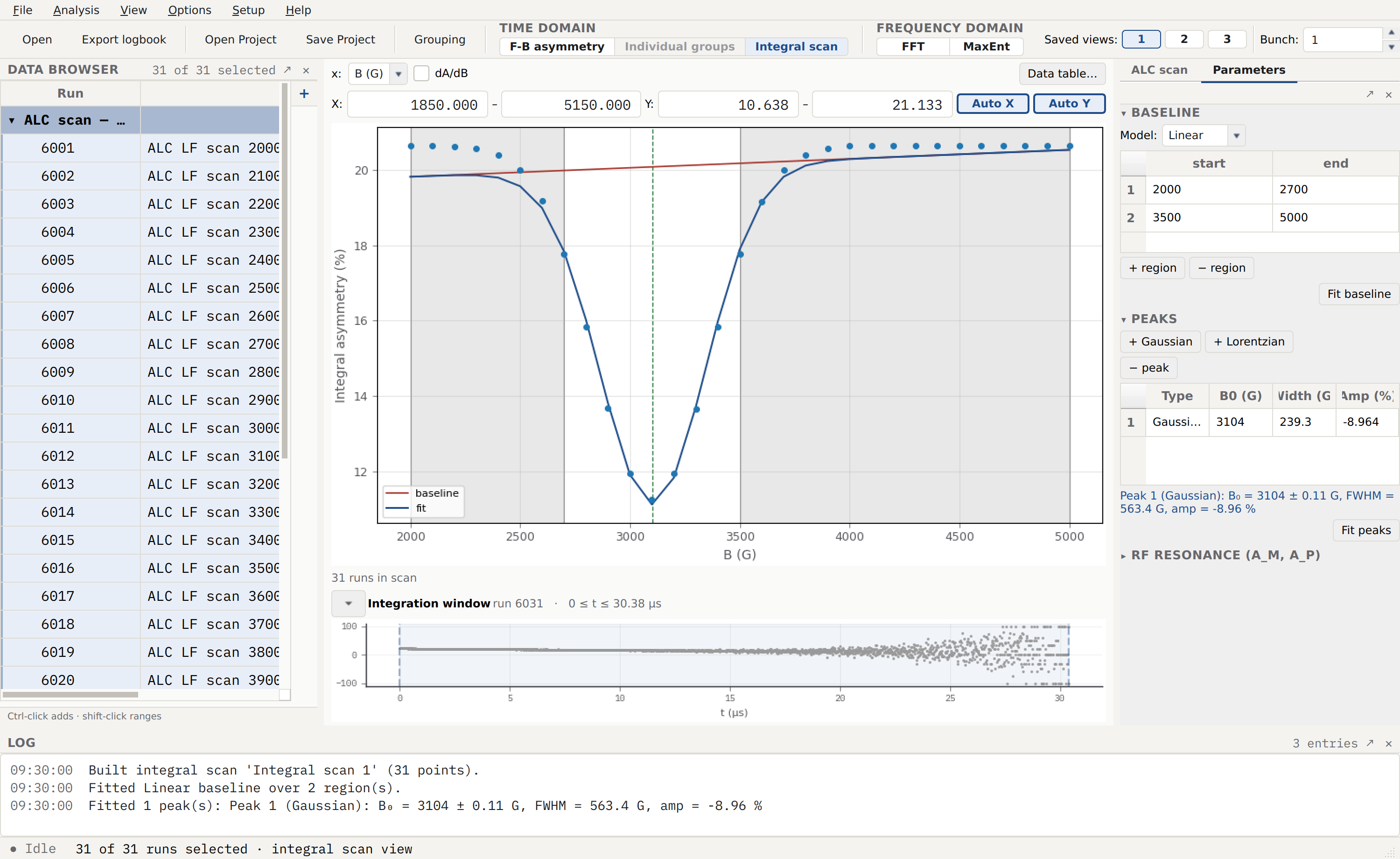
The steps mirror a real analysis:
Load the field-stepped runs and select them all.
Switch the toolbar to the Integral scan representation and, in the Fit dock, press Build Scan — each run is integrated over the time window to a single point, and the scan of integral asymmetry against field appears in the central plot area.
Mark two non-resonant field regions either side of the dip and press Fit baseline (a straight line here).
Add a Gaussian peak and press Fit peaks. The fit recovers the resonance field — \(B_0 \approx 3104\) G, against the 3100 G the scan was built with — along with its width and amplitude.
For the same workflow on real data, see ALC field scan in TCNQ.
Common pitfalls
The scan area is empty after entering the representation. The scan is built, not automatic: multi-select the runs, set the integration window, and press Build Scan in the Fit dock. Until then the central area shows the “Build a scan to see the ALC curve” placeholder.
A run is missing from the scan. Field-axis scans drop runs with no recorded field (and likewise for temperature); the provenance line beneath the scan names them (and its tooltip gives the reason), or switch the x-axis to Run.
A point is greyed and hollow. You (or a saved project) excluded that run by clicking it — click it again to restore it. The provenance line tells you how many points are excluded this way.
“Add at least one non-resonant region”. The baseline needs at least one region, and a Linear baseline needs at least two usable points across the marked regions. Widen the regions or use a Constant baseline.
Regions or peaks disappeared. Changing the x-axis clears them, because they are expressed in the units of the axis they were drawn on.
The baseline or fit overlay vanished after an edit. Editing a region or dragging a handle marks the fit stale on purpose; press Fit baseline (and then Fit peaks) again.
Further reading
F. L. Pratt, WiMDA: a muon data analysis program for the Windows PC, Physica B 289–290, 710 (2000). — the count-integral ALC this mode follows.
The Mantid
PlotAsymmetryByLogValuealgorithm — the alpha-aware integral/differential field-scan reference.
See also
Fitting engine — time-domain model fitting (the per-spectrum alternative).
Parameter trending — trending fitted parameters across a run series.
Detector Grouping and Layout — the F/B grouping and \(\alpha\) used by the integral.
Project files — what is saved in a project and how it is restored.