ALC field scan in TCNQ

An avoided-level-crossing (ALC) measurement asks a different question from a time-domain relaxation fit. Instead of following one spectrum in time, it steps the applied longitudinal field through a resonance and watches a single reduced number — the time-integral asymmetry — dip as the field crosses the level anticrossing. The dip field pins a hyperfine coupling, and its width and temperature dependence report on molecular motion. This chapter builds that scan end-to-end on the real muon-school TCNQ data, fits the resonance, and reads the muon hyperfine coupling off it; a closing advanced section carries the same workflow to a four-resonance corannulene spectrum published to sub-percent precision.

The Integral scan mode is Asymmetry’s home for this analysis: it reduces every run to one integral-asymmetry value and plots it against the swept field, then lets you fit a baseline and resonance peaks to the resulting curve. For the full feature reference — the differential view, project persistence, and the scripting entry points — see Integral scan mode (avoided-level-crossing field scans); this page is the worked walkthrough on real data.

The runs

The corpus Chemistry → ALC resonance in TCNQ set is a longitudinal-field study of a muoniated TCNQ radical — the muonium adduct formed when muonium adds to tetracyanoquinodimethane, an organic electron acceptor — measured on EMU at the ISIS pulsed muon source. The muon is proposed to sit on the nitrogen of a cyano group, and the object of the experiment is its hyperfine coupling and how motion averages it.

The folder holds 128 EMU .nxs runs (emu00019485–emu00019612) organised as four field scans, each 31 runs stepped from 2000 to 5000 G in 100 G steps, repeated at setpoint temperatures 350 / 100 / 50 / 10 K. The worked example below builds the 350 K scan first (runs 19489–19519), then overlays all four. Each run’s swept field is read from its metadata, so the Data Browser resolves a B (G) column automatically and the scan’s field axis needs no hand entry.

Note

The instrument stores the setpoint temperature; the cryostat drifts a little from it (the 350 K scan measures ≈ 338–343 K, and the first two 10 K runs are still settling at ≈ 10–11 K). Scans are labelled by setpoint throughout, with the measured temperature logged per run.

Building the integral scan

1. Load the scan and select it. Open the 31 runs of the 350 K scan and multi-select them in the Data Browser — click the first row, then Shift-click the last. The scan is built from the selected runs, exactly as a batch fit is.

2. Enter the Integral scan representation. Click Integral scan in the Time domain cluster of the main toolbar. The central plot area switches to the scan view; the fit dock’s ALC scan tab shows the Integral scan (ALC) build panel, and its Parameters tab shows the Baseline, Peaks, and RF resonance (A_µ, A_p) sections.

   Note

   Integral scan is always available — the two-or-more-runs requirement is checked when you build the scan, not on the toolbar button.

3. Set the integration window and build. The Integration window is the time window each run’s asymmetry is integrated over. Drag the shaded window on the slim time-spectrum strip beneath the scan, or type \(t_\mathrm{min}\) and \(t_\mathrm{max}\) into the spinboxes, then click Build Scan. Each selected run collapses to one point and the scan appears in the central area.

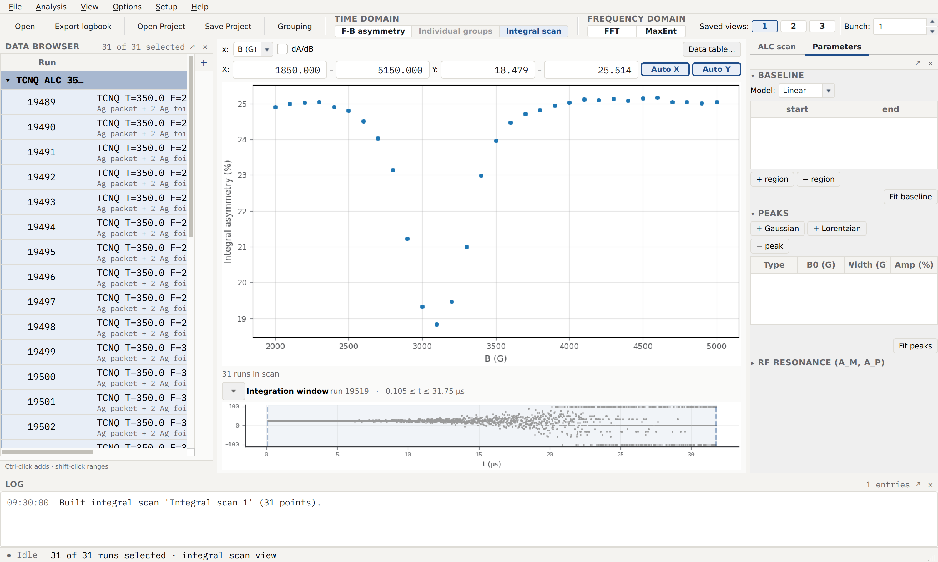
The raw 350 K scan, freshly built. The 31 selected runs (19489–19519) have each been reduced to one integral-asymmetry value and plotted against B (G): a flat ≈ 25 % baseline off resonance collapses into a clean D1 dip near 3100 G. The provenance line reads 31 runs in scan and the log confirms Built integral scan ‘Integral scan 1’ (31 points). The integration-window strip below shows this scan taken over the full good-time window (\(0.105 \le t \le 31.75\) μs) of run 19519; the Baseline and Peaks panels on the right are still empty, because the scan is the model-free observable and the fitting comes next.

Note

The integral here is the WiMDA count integral — forward and backward counts are summed over the window before the asymmetry ratio is formed, so the value is Poisson-weighted across the whole window and is invariant to the display bunching. The teaching guide reaches the same scan by setting a bunch factor of 500 (≈ 4 μs display bins); that is a WiMDA display convenience and does not change the summed-count integral.

Fitting the resonance

With the scan built, the two-step ALC fit lives in the Parameters tab. A resonance sits on a smoothly varying non-resonant background, so it is fitted in two stages — subtract the baseline, then fit the peak on what remains.

1. Fit a baseline. In the Baseline section choose the Model — Cubic here, the curved WiMDA/Mantid ALC background a straight line cannot match — then press + region twice and enter the two non-resonant windows that bracket the dip, 2000–2600 G and 3400–5000 G (type them, or drag the shaded region edges on the plot). Press Fit baseline.

2. Fit the resonance peak. In the Peaks section press + Lorentzian to add a peak, seed its B0 (G), Width (G), and Amp (%) near the dip (say 3050 G, 140 G, −5 %), and press Fit peaks. The total fit — baseline plus peak — is overlaid on the scan and the read-out below the peaks table reports the fitted resonance field, width, and amplitude.

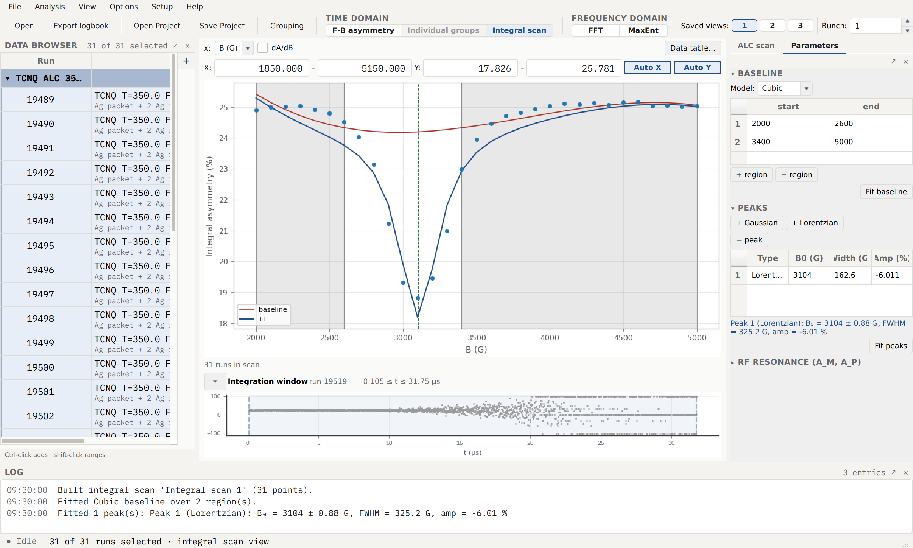
The converged fit. The Cubic baseline (red) is fitted over the two shaded non-resonant regions and the Lorentzian (blue total) traces the D1 dip; the green dashed line marks the fitted centre. The read-out and log agree: Peak 1 (Lorentzian): B₀ = 3104 ± 0.88 G, FWHM = 325.2 G, amp = -6.01 %. The Lorentzian slightly over-peaks the very bottom of the dip — the true line is a touch rounder — but the centre is pinned to better than a gauss, which is what the hyperfine coupling depends on.

Note

The teaching guide names a two-Lorentzian model, but only a single genuine D1 resonance sits in this window; the second line is a template default and, left in, would be unconstrained. Fitting one Lorentzian is the physically correct choice and gives the well-determined centre above. A truly overlapping pair of resonances does need a joint fit — that case appears in the corannulene section below.

From resonance field to hyperfine coupling

The dip is the D1 (\(\Delta M = \pm 1\)) avoided-level crossing of the muon–electron system. Its field is set by the muon hyperfine coupling \(A_\mu\) through

\[B_\mathrm{res} = \frac{A_\mu}{2}\left(\frac{1}{\gamma_\mu} - \frac{1}{\gamma_e}\right),\]

where \(\gamma_\mu\) and \(\gamma_e\) are the muon and electron gyromagnetic ratios. Inverting it turns the fitted centre straight into the headline number: with \(\gamma_\mu^{-1} - \gamma_e^{-1} = 73.42\) G MHz⁻¹,

\[A_\mu\,[\mathrm{MHz}] \approx \frac{B_\mathrm{res}\,[\mathrm{G}]}{36.71},\]

so the 350 K resonance at \(B_\mathrm{res} = 3104\) G gives

\[A_\mu \approx 84.6\;\mathrm{MHz}.\]

The guide sets the radical up to sit near \(A_\mu \approx 80\) MHz — a resonance near \(B_\mathrm{res} \approx 2937\) G — and that is the value to sanity-check against, the “expected neighbourhood” rather than an answer key. The fitted 84.6 MHz is the deliverable: the precise coupling is read off the fit, and it lands within a few percent of the nominal target, closing on it as the sample cools (the 10 K scan gives 81.9 MHz).

Why the resonance sits at \(B_\mathrm{res} = (A_\mu/2)(\gamma_\mu^{-1}-\gamma_e^{-1})\)

In a muoniated radical the muon (spin \(I_\mu\)) and the unpaired electron (spin \(S\)) are coupled by an isotropic hyperfine interaction \(A_\mu\,\mathbf{I}_\mu\!\cdot\!\mathbf{S}\), and both precess in the applied longitudinal field \(B\). At high field the good quantum numbers are the Zeeman projections \(m_\mu\) and \(m_S\). Two levels of the spin manifold that differ by \(\Delta M = \pm 1\) — a simultaneous muon and electron spin flip, \(\Delta m_\mu = +1\), \(\Delta m_S = -1\) — approach each other as the field is swept, because the muon and electron Zeeman energies change with opposite sign relative to the hyperfine splitting.

Setting the two Zeeman contributions equal and opposite about the hyperfine term, the near-degeneracy is reached when

\[\gamma_\mu B_\mathrm{res} + \gamma_e B_\mathrm{res} \;\text{balances}\; A_\mu,\]

which rearranges to the resonance condition above, \(B_\mathrm{res} = (A_\mu/2)(\gamma_\mu^{-1} - \gamma_e^{-1})\). The isotropic (hyperfine) part of the coupling therefore fixes where the crossing is (hence \(A_\mu\)), while the anisotropic (dipolar) part is what actually mixes the two levels — turns the true crossing into an avoided crossing — and so sets the width of the dip. That is why the same scan yields two physical numbers: the centre for \(A_\mu\) and the width for the dipolar coupling \(D_\mu\), taken up next. For the D1 line with axial dipolar symmetry the guide relates the two by \(\mathrm{FWHM}\,[\mathrm{G}] \approx 68\,D_\mu\,[\mathrm{MHz}]\).

The temperature series: motional narrowing

Repeating the build-and-fit at all four temperatures turns one number into a story about dynamics. Overlaying the scans shows the dip changing shape systematically with temperature.

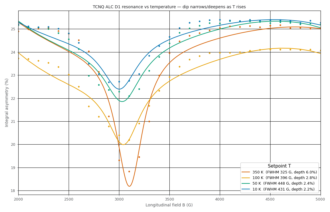
All four field scans overlaid, warm (350 K, vermillion) to cold (10 K, blue), each drawn with its fitted Lorentzian-plus-cubic curve. As the sample warms the D1 dip deepens and narrows — the legend carries each scan’s FWHM and depth (350 K: FWHM 325 G, depth 6.0 %; down to 10 K: FWHM 431 G, depth 2.2 %). A narrowing resonance with rising temperature is the signature of motional averaging: as molecular motion speeds up it averages the anisotropic (dipolar) part of the hyperfine tensor towards zero, so the line the muon sees narrows.

The width converts to the muon dipolar coupling through the guide’s D1 relation, \(D_\mu\,[\mathrm{MHz}] = \mathrm{FWHM}\,[\mathrm{G}]/68\). Trending \(A_\mu(T)\) and \(D_\mu(T)\) together is the hyperfine deliverable of the whole experiment.

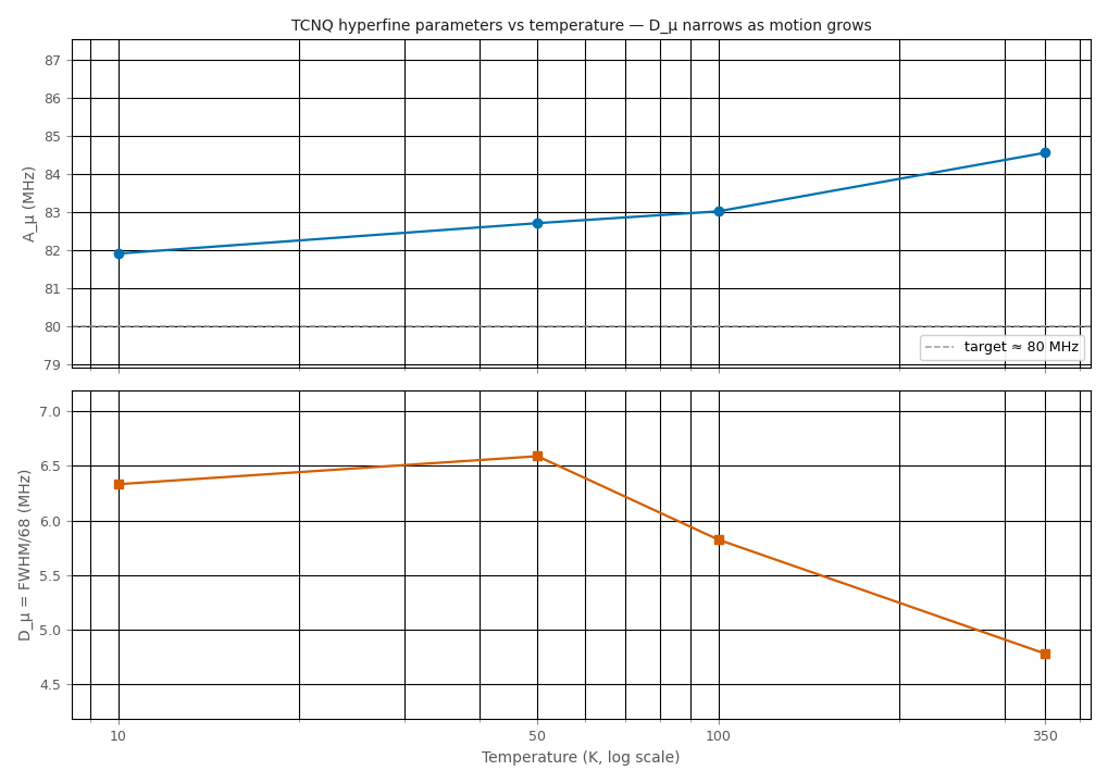
The hyperfine parameters versus temperature. The muon coupling \(A_\mu(T)\) (top) stays close to the ≈ 80 MHz target across the whole range, edging up from 81.9 MHz at 10 K to 84.6 MHz at 350 K. The dipolar coupling \(D_\mu(T)\) (bottom) falls as the sample warms, from ≈ 6.3 MHz cold to 4.8 MHz at 350 K — the dipolar tensor being motionally averaged as molecular motion grows, the answer to the guide’s question about what dynamics the radical undergoes. The trend is cleanest above 50 K; the 10 K point breaks strict monotonicity, consistent with its first runs still settling in temperature.

Scripting the scan

The GUI build panel calls the same core builder your scripts can use. build_field_scan() integrates every run over the window and returns the sorted scan; fit_scan_baseline() and fit_scan_model() reproduce the Baseline and Peaks buttons:

from glob import glob

import numpy as np
from asymmetry.core.io import load
from asymmetry.core.transform.integral import build_field_scan
from asymmetry.core.fitting.field_scan import fit_scan_baseline, fit_scan_model

scan_files = sorted(glob(".../ALC resonance in TCNQ/Data/emu000195*.nxs"))
runs = [load(p) for p in scan_files[:31]]   # the 31 field-stepped 350 K runs
scan = build_field_scan(runs, method="integral", order_key="field")

b_dip = scan.x[int(np.argmin(scan.value))]
print(round(float(b_dip)))                  # 3100  (G, the raw minimum)

# Cubic baseline over the non-resonant edges, then a Lorentzian on the dip:
base = fit_scan_baseline(scan, [(2000.0, 2600.0), (3400.0, 5000.0)], model="Cubic")
fit = fit_scan_model(base.corrected, ["LorentzianLCR"],
                     initial={"f": -3.0, "B0": 3100.0, "Bwid": 120.0})
b_res = float(fit.parameters["B0"].value)
print(round(b_res / 36.71, 1))              # 84.6  (A_µ in MHz)

The raw minimum falls on the 3100 G point, and the fitted Lorentzian centre (3104 G) inverts to \(A_\mu \approx 84.6\) MHz — the GUI result reproduced from a script.

Advanced: a four-resonance µLCR spectrum

The TCNQ scan has one resonance; the technique scales to several. The corpus Chemistry → Molecular dynamics of corannulene set is the flagship example — and it is paper-graded: the runs are the very data of Gaboardi et al., Carbon 155, 432 (2019) (the NeXus headers carry that experiment’s beamtime award and the paper’s own author list). Corannulene, C₂₀H₁₀, is a cup-shaped polycyclic aromatic hydrocarbon — roughly one third of a C₆₀ ball — that chemisorbs muonium to form four long-lived muoniated-radical adducts, R1–R4, each with its own muon hyperfine coupling and so its own µLCR resonance.

The widest scan in the corpus

The measurement is a µLCR (muon level-crossing resonance) field scan on the HiFi spectrometer, run at two temperatures whose measured sample values are the paper’s 40 K (setpoint 50 K) and 410 K (setpoint 420 K). The 40 K wide scan alone is 158 runs stepped from 0.5 to 3.0 T — the widest field scan in the whole corpus — built in the Integral scan view exactly as the TCNQ scan was.

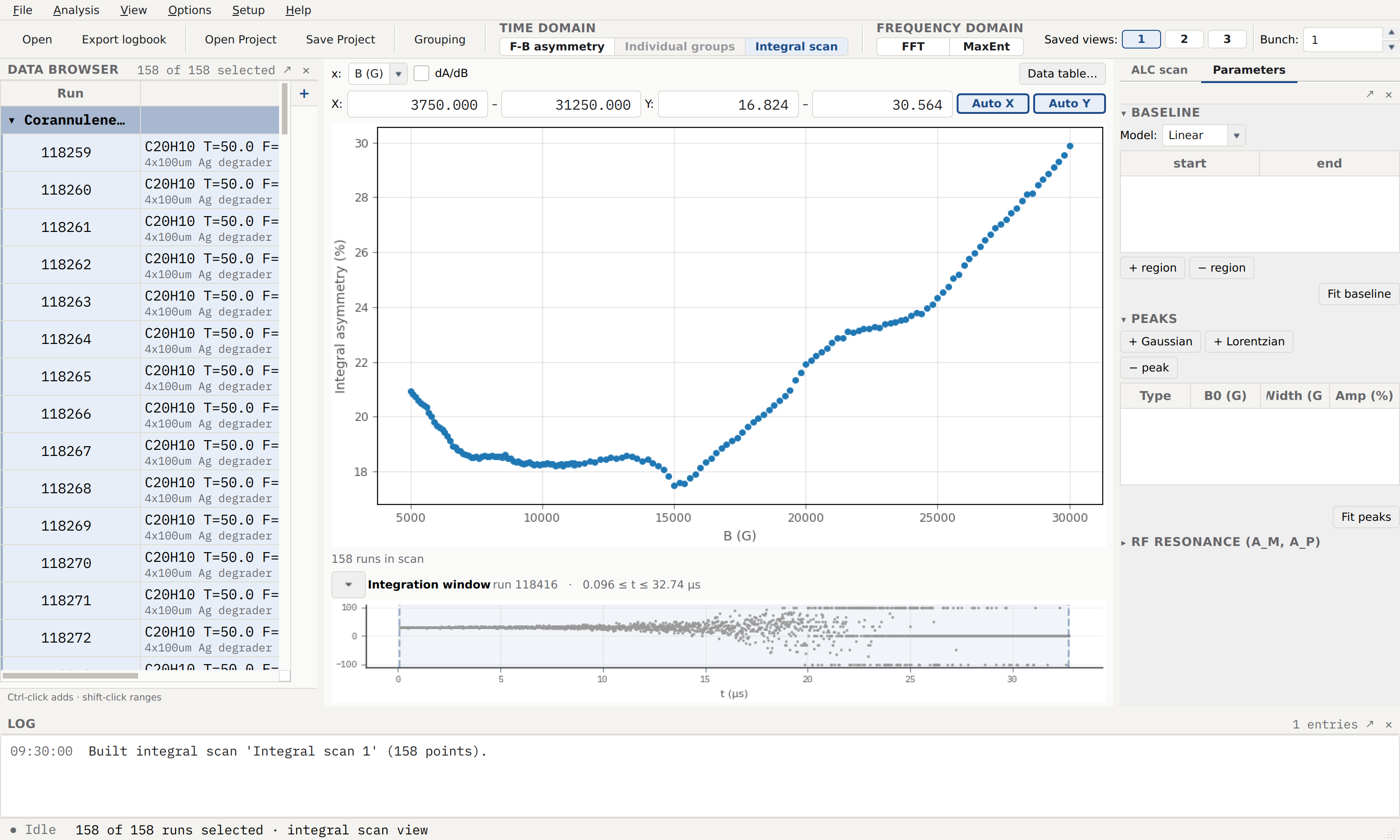
The 40 K corannulene scan in the Integral scan view: 158 HiFi runs (118259–118416) reduced to integral asymmetry against longitudinal field over 0.5–3.0 T. Unlike the flat TCNQ baseline, here the integral asymmetry rises steadily across the whole scan — the broad longitudinal- field repolarisation envelope of muonium — with the strong R3 resonance dip carved out of it near 15000 G (1.53 T). Fitting on a background this curved is what the higher-order polynomial baselines (a Quartic here) are for.

Four resonances, four hyperfine couplings

Subtracting the repolarisation background and fitting the four \(\Delta M = \pm 1\) dips turns the spectrum into four hyperfine couplings. Each fitted resonance field inverts through the same relation as before, \(A_\mu\,[\mathrm{MHz}] = B_\mathrm{r}\,[\mathrm{G}]/36.713\).

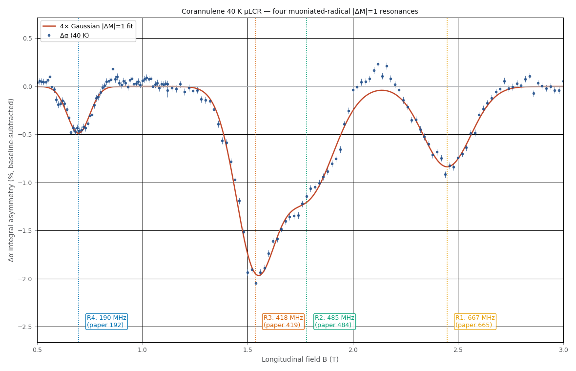
The background-subtracted 40 K spectrum (Δα) with the four \(\Delta M = \pm 1\) resonances fitted as Gaussian lines. Reading the coupling off each fitted centre gives \(A_\mu = 190 / 418 / 485 / 667\) MHz for R4 / R3 / R2 / R1 — set against the paper’s Table 1 values of 192(11) / 419(10) / 484(20) / 665(15) MHz, every one lands inside the published 1σ uncertainty. That is the flagship precision result of the corpus: four independent hyperfine couplings reproduced to the paper’s own error bars from a single reduced scan.

Tip

R2 and R3 overlap, and must be fitted jointly. The two central lines (≈ 1.53 T and ≈ 1.8 T) sit close enough that their wings merge into one shoulder. Fitting them one at a time is unreliable — a single line dropped on the R2 window collapses onto the stronger R3 — so they are fitted together as a two-Gaussian doublet in one minimisation, which separates the shoulder cleanly. The outer lines R4 and R1 are well isolated and fit singly. This is the general rule for overlapping resonances: one shared fit, not sequential passes (see Integral scan mode (avoided-level-crossing field scans) for the multi-resonance API).

Molecular dynamics: what warming does to the lines

The whole point of the two temperatures is the contrast between them. Overlaying the 40 K and 410 K subtracted scans shows each resonance responding differently to the onset of molecular motion.

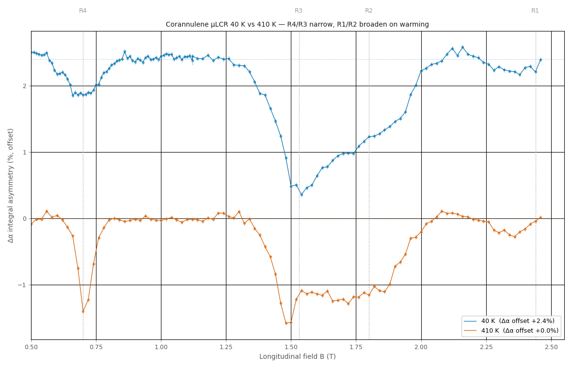
The 40 K (blue, offset up) and 410 K (vermillion) scans overlaid, in the style of the paper’s Fig. 4. On warming, the two low-field lines R4 (0.7 T) and R3 (≈ 1.5 T) narrow into sharp needles — R4’s width drops by roughly a factor of four — while the higher-field R1 (2.44 T) all but vanishes and R2 weakens and broadens. The narrowing is the signature of fast molecular rotation switching on (a pre-melting state): rotation about the five-fold symmetry axis averages the dipolar tensor of the sites whose coupling lies along it, sharpening R3 and R4, while the less favourably oriented R1/R2 sites broaden instead.

A complementary muonium fingerprint: repolarisation

The same runs at low field give a second, independent measurement. A longitudinal-field repolarisation curve plots the recovered muon polarisation against field: as the field decouples the muon from its electron, the polarisation climbs through a step whose size is the muonium fraction.

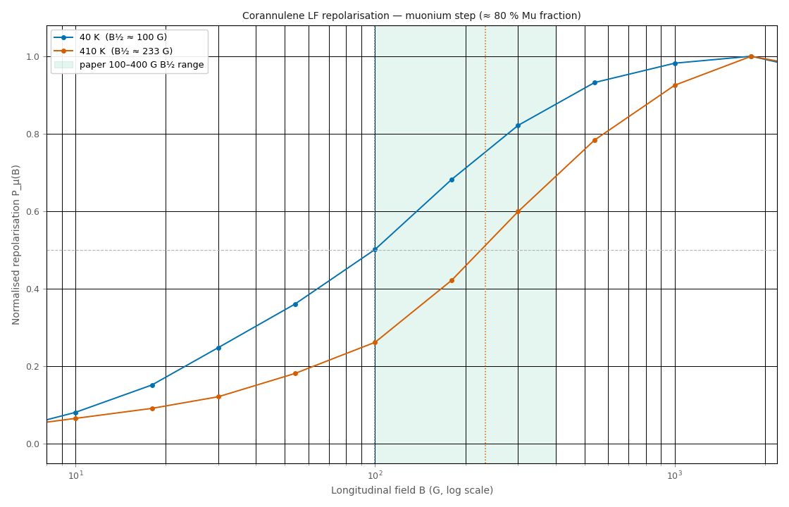
The low-field repolarisation curves at 40 K and 410 K (log field). Both climb through the muonium step that signals ≈ 80 % of implanted muons forming muonium, and the half-repolarisation field \(B_{1/2}\) — where the curve crosses halfway — moves from ≈ 100 G at 40 K to ≈ 233 G at 410 K, both inside the paper’s stated 100–400 G range (shaded). The shift to higher field on warming means the polarisation is recovered more slowly, a complementary readout of the same hyperfine physics the µLCR dips measure directly.

Assumptions and limitations

• The fitted coupling is the deliverable, not the nominal target. The TCNQ guide’s ≈ 80 MHz (≈ 2937 G) is the expected neighbourhood the radical is set up to occupy; the precise \(A_\mu\) is read off the fitted resonance centre. The fitted 82–85 MHz across the four scans is a legitimate result, not a miss.

• The number of genuine resonances is a physics judgement. A template may name more lines than the data support (TCNQ’s “two Lorentzians”), or fewer than overlap demands (corannulene’s merged R2/R3). Fit the resonances the data actually resolve, and fit overlapping ones jointly.

• The baseline model is a choice. A curved non-resonant background needs a polynomial baseline (Cubic for TCNQ, Quartic for the steep corannulene repolarisation envelope); too low an order leaves residual curvature under the peaks, and too high an order can overshoot between resonances. The four corannulene dip positions are robust to a small over-shoot of the Quartic between R1 and R2, but a precise depth or area would not be.

• Absolute amplitudes are not graded. The corannulene paper plots µLCR signals in arbitrary units with the two temperatures offset, and the repolarisation step here is normalised to its high-field plateau — so the positions and widths (hence the couplings and the narrowing contrast) are the reproduced quantities, not absolute dip depths or the absolute 0.80 muonium fraction.

• Field geometry labelling. These scans are longitudinal-field sweeps, though the corannulene NeXus metadata mislabels the field state; the applied-field magnitude used for the scan axis is reliable.

References

• M. Gaboardi, F. L. Pratt, C. Milanese, J. Taylor, J. Siegel, and F. Fernandez-Alonso, Carbon 155, 432 (2019) — the published µLCR study of corannulene reproduced in the advanced section: four muoniated-radical hyperfine couplings and their motional narrowing.

• F. L. Pratt et al., Magn. Reson. Chem. 38, S27 (2000) — muonium addition to TCNQ and the muoniated radical.

• R. M. Macrae, Magn. Reson. Chem. 38, S33 (2000) — the ab initio assignment of the muon addition site on TCNQ.

• E. Roduner, Chem. Soc. Rev. 22, 337 (1993) — the ALC-µSR technique and the D1 resonance condition.

• F. L. Pratt, Physica B 289–290, 710 (2000) — WiMDA, whose count-integral ALC the Integral scan mode follows.

• S. J. Blundell, R. De Renzi, T. Lancaster, and F. L. Pratt, Muon Spectroscopy: An Introduction (Oxford University Press, Oxford, 2022), Ch. 6 — muonium, radicals, and avoided-level-crossing spectroscopy.

Cross-references

• Integral scan mode (avoided-level-crossing field scans) — full Integral scan (ALC) reference: the baseline and peak fitters, the differential dA/dB view, the RF-resonance (Green − Red) observable, the multi-resonance fitting API, and project persistence.

• EMU detector grouping and α calibration — the grouping and \(\alpha\) setup shared by every run in a scan.

• Parameter trending — the complementary route for a smooth repolarisation curve, fitting a MuRepolarisation model for the hyperfine constant directly.

• Composite models — building the composite Gaussian / Lorentzian-plus-polynomial models a multi-resonance scan is fitted with.