Detector Grouping and Layout
Detector grouping defines how the raw per-detector count histograms are combined into the forward and backward sums that enter the asymmetry formula. The choice is dictated by the experiment: a coarse two-group arrangement is right for ordinary asymmetry analysis on a longitudinal spectrometer; keeping detectors as individual groups is what enables the per-detector amplitudes and phases needed for a paramagnetic Knight-shift measurement (Grouped time-domain fitting); and a vector-polarisation experiment needs distinct pairs assigned to \(P_x\), \(P_y\), and \(P_z\) (Vector-polarisation mode). For new data from any of the supported instruments — ISIS HiFi, MuSR, EMU and the PSI FLAME, HAL-9500 and GPS spectrometers — the matching preset in the Detector Layout editor seeds sensible defaults that can then be refined graphically before being applied.
Grouping is configured from the Grouping window and edited graphically with the Detector Layout editor. This page covers both, together with the grouping-profile model that stores the settings, the per-format (PSI/ROOT) details, and the beam-vs-analysis naming conventions. For a hands-on walkthrough with a worked calibration, see Grouping and calibration walkthrough.
Grouping profiles
A grouping profile is a named, project-level record of the shareable grouping settings for one instrument — the detector groups, which pair is forward/backward, the \(\alpha\) policy, and the deadtime, background, binning and period settings. It excludes anything that is a fact about an individual run rather than a shared analysis choice: \(t_0\), the good-bin window, per-detector deadtime read from a file, and period tables stay with the run.
This split solves a real problem. Every run used to carry its own complete grouping payload, so recalibrating \(\alpha\) after loading a fifth run in a series meant editing it a fifth time — and nothing stopped two runs of the same series from silently drifting apart. A profile fixes the shareable choices in one place: edit it once, and every run that matches it is analysed the same way.
Instrument and scope
A profile applies to every run of one instrument — matched, internally, on
the pair (instrument, histogram count). The histogram count disambiguates
layout variants of the same physical instrument, such as PSI GPS’s
six-detector PSI-BIN export and eleven-detector MusrRoot export (see PSI GPS
below): both are shown as one instrument, but a GPS PSI-BIN profile is never
offered to an eleven-detector GPS ROOT run. The window names the instrument
plainly — “GPS” — and appends the detector count only when two variants of the
same instrument are both loaded, so they can be told apart: “GPS (6 detectors)”
and “GPS (11 detectors)”.
A project may hold several profiles per instrument in concurrent use — the typical case is one profile per sample, each with its own background, \(\alpha\), and deadtime settings, kept in one project so the samples can be compared side by side. Every run records which profile it is assigned to and follows that profile; editing a profile reaches exactly the runs assigned to it and leaves the other profiles’ runs alone. One profile per instrument is flagged the default for new runs (marked ★ in the Grouping window’s profile selector): a newly loaded run is assigned to it automatically — no per-run Apply step is needed — and can then be reassigned to another profile, from the Grouping window’s scope panel or the Data Browser’s Assign Grouping Profile context menu (Assigning runs to profiles below).
Because a run’s instrument is a fact about its data rather than a user preference, a stale persisted instrument identity self-heals on reload: if a project saved the wrong instrument for a run (for example, a FLAME run stored as “GPS” by an older version), re-detection from the freshly loaded file overrides the stored value, the run is re-matched to the correct instrument’s profile (or kept on the loader defaults if none exists), and the mismatched preset’s group names are discarded. Saved profiles themselves are never altered — only runs heal.
A run can be explicitly released from its profile, freezing its current grouping as a per-run override that further profile edits do not touch. The Data Browser marks a released run with a trailing ⊗ and the tooltip “Custom grouping — this run is released from its grouping profile (based on ‘<profile>’).” — the named profile is the run’s base, the one it stays assigned to while released. A released run can later be reattached, dropping the override so it follows its base profile again. Release and reattach are both driven from the Grouping window’s scope panel (The Grouping window below).
Assigning runs to profiles
Which profile a run follows is an explicit, per-run assignment. It can be changed in two places, and both apply the target profile’s settings to the moved runs immediately:
Grouping window — select runs in the scope panel and press Assign to ▸, which lists every profile of the instrument. Assigning a released run does not drop its override; it only retargets the base profile that Reattach returns it to.
Data Browser — select any number of runs and choose Assign Grouping Profile from the context menu; the runs’ current profile is checked. The submenu appears once the selected runs’ instrument has at least two profiles.
Every non-default profile of a multi-profile instrument carries its own identity colour, assigned from a fixed palette when the profile is first saved and stored with it in the project; the ★ default profile stays uncoloured, so its runs keep plain black run numbers and a coloured run number always means “assigned off the default”. The colour is worn consistently everywhere the profile appears: the Data Browser colours each run’s number with its assigned profile’s colour (with the tooltip “Grouping profile: <name>” naming it), the Grouping window’s scope rows, editing strip, and selector swatches use the same colour, and a released run shows amber instead — the diverged state outranks sample identity. A multi-sample project therefore reads as a colour-coded sample map; single-profile projects stay entirely uncoloured.
Alpha, deadtime, and background policies
A profile stores each of its three corrections as a policy — a mode plus whatever value the mode needs — rather than a bare value, so the provenance of the number survives:
Alpha policy —
fixedapplies the same value to every run;calibratedapplies a value measured once (with a recorded method and source run, e.g. “diamagnetic · run 2923”);per_run_estimatecomputes each run’s own forward/backward integral ratio at resolution time (Mantid’sAlphaCalc; the PSI.bindefault), so a series with detector sensitivities that drift run-to-run stays self-consistent without a shared number.Beta — the intrinsic-asymmetry balance \(\beta = A_{0,b}/A_{0,f}\) (musrfit’s asymmetry-fit companion to \(\alpha\)), stored as a plain fixed scalar and applied with \(\alpha\) in the asymmetry formula \(A = (F - \alpha B)/(\beta F + \alpha B)\). The default 1 is the standard formula and is omitted from saved profiles, so existing projects are unaffected. There is no estimator — \(\beta\) scales the asymmetry amplitude, not the count rate, so no count ratio can measure it.
Deadtime policy —
offdisables the correction;from_filereads each run’s own file deadtime values;manualapplies a stored per-detector table (hand-typed or fitted with Cal);estimateapplies one fitted value to every detector.Background policy —
none,range(a pre-\(t_0\) window),tail_fit(a late-time Poisson fit),reference_run(a dedicated background run), orfixed(constant forward/backward values). See Background Correction below for the maths each mode applies.
Resolving a profile against a run merges these policies with the run’s own
file-derived facts to produce exactly the same grouping payload shape used
before profiles existed, so nothing downstream — reduction, fitting, export —
had to change to support them. The reduction itself funnels through one
function, asymmetry.core.transform.reduce.reduce_grouped_asymmetry(),
which applies deadtime correction, groups the histograms onto a common
\(t_0\), optionally subtracts background, and forms the counts-then-ratio
asymmetry — the same order the Grouping window’s live preview and the main
reduction path both use, so what you see while editing is what you get after
Apply.
Migration from older projects
Projects saved before profiles existed (schema v11 and earlier) store a complete grouping payload on every dataset. Opening such a project migrates it to schema v12 automatically: datasets are grouped by instrument, and within each instrument
if every run’s shareable settings already agree, one active profile named “Default (<instrument>)” is created and every contributing run switches from its own payload to a reference to that profile;
if the shareable settings disagree, a profile is built from the majority payload; runs matching it inherit the profile, and the remaining, genuinely divergent runs keep their per-run payload untouched, exactly as a manually released run would.
The migration is additive: nothing that could not be faithfully represented as a profile is discarded, and a run whose instrument cannot be identified (missing instrument metadata) is left with its original payload and joins no profile.
Projects from before assignments were explicit (schema v16 and earlier, where each instrument had a single active profile that runs inherited implicitly) migrate to schema v17 by recording each run’s assignment: a run that named a profile keeps it as its explicit assignment, and a released run additionally records the instrument’s active profile as its base — the reattach target — while keeping its override payload untouched. The behaviour of a single-profile project is unchanged. Saving the project afterwards writes the current schema (see Project files).
The Grouping window

The Grouping window’s profile editor, with the scope panel on the left and the live forward/backward asymmetry preview along the bottom. Two sample profiles are in concurrent use: “Sample A” (the ★ default, being edited) and “Sample B”, with one run following each.
Open it with the Grouping button on the main toolbar (or Analysis → Grouping…). Where the old dialog operated on a reference run and broadcast settings to whichever datasets were checked, the window is now a profile editor: it edits one profile’s settings in a draft, and that draft is what gets applied to every run following the profile.
Profile selector — switches which saved profile is being edited, and offers New… and Duplicate… to start a fresh profile or branch one from the current settings (a new profile starts with no runs assigned — assign them from the scope panel). Only profiles for the selected instrument are listed — non-default profiles with their identity-colour swatch, and the instrument’s default-for-new-runs profile marked ★. Switching away from a profile with unsaved edits prompts to discard them.
Rename… renames the edited profile in place — the stored profile is replaced under its new name on Apply and every run’s assignment follows; a name already used by another profile of the instrument is refused. Delete… removes the edited profile: if runs are assigned to it you choose which remaining profile they move to, and the last profile of an instrument cannot be deleted. A Default for new runs checkbox makes the edited profile the instrument’s default on Apply; it cannot be unchecked directly — defaultness moves by checking it on another profile — and saving a profile never steals the default on its own.
Instrument switcher (“Instrument”) — chooses which instrument’s profile the window edits, listing every instrument present in the loaded datasets as “GPS — 3 runs”. It is hidden when the project holds a single instrument, since there is then nothing to switch between. Picking another instrument swaps the whole editor — its draft, selected run, scope panel, and preset list all follow — after the same discard prompt the profile selector uses for unsaved edits.
Scope panel — the selector. Headed “Runs of this instrument”, it lists the runs of the selected instrument, each tagged follows <profile> (its assigned profile, in that profile’s identity colour; the ★ default’s rows stay plain — the edited profile’s runs additionally bold on a soft tint of the same colour, or of the standard accent while editing the default) or override (amber, with the base profile appended as override · <profile> when it is not the edited one). Release from profile, Reattach to profile, and Assign to ▸ buttons move the selected runs between those states. The run selected here is the one the form previews and edits: selecting a run shows that run’s effective settings in the form, drives the live preview, and seeds the status rows with its per-run facts (\(t_0\), good-bin window, file deadtime, period tables). What your edits change follows the selected run’s status (Editing target follows selection below). Apply is disabled only when nothing would be committed: no run follows the edited profile, no override has pending edits, and no reassignment, rename, deletion, new profile, or default change waits.
Editing-target strip — right-aligned in the dialog’s top row, a persistent strip states what your edits currently apply to: “Editing profile ‘<name>’ — applies to N runs”, in the edited profile’s identity colour (the standard accent while editing the uncoloured ★ default), while a following run is selected, or warning-tinted “Editing override for run N — this run only” while an overridden run is selected. The same tint highlights the selected row in the scope list, and a run with uncommitted override edits gains an “override *” marker there.
Preset dropdown and chip — an instrument-aware preset dropdown in the left column, directly above the group table it seeds with a sensible starting arrangement (see the per-instrument sections below), and a chip beside it reads either “Preset: <name>” when the draft’s groups still match that preset exactly, or “Custom (edited from <name>)” the moment any group, name, or forward/backward assignment is edited by hand. This comparison is re-made every time the draft changes rather than cached, so the chip never keeps showing a preset name the settings have since drifted away from.
Live asymmetry preview — a debounced plot of the forward/backward asymmetry the current draft would produce on the selected run, recomputed automatically as groups, \(\alpha\), binning, deadtime, or background settings change. The recompute runs on a worker thread (never the GUI thread), so editing stays responsive even while a reduction is in flight; a superseded recompute is discarded in favour of the latest edit.
Two-column settings — the right pane is a full-width pipeline strip over two side-by-side columns, with the compare controls and the live preview pinned below both. The Grouping and timing column (left) holds the groups, t0, binning, exclusions and periods; the Corrections column (right) holds four collapsible correction cards — Deadtime, Background, α (detector balance) (its value and provenance or, in vector mode, the per-projection table, plus the calibration controls), and β (asymmetry balance) (a fixed β value entry for musrfit’s intrinsic-asymmetry balance; hidden in vector mode, where per-projection reductions stay at β = 1) — each previewed against the same corrected reduction. A card’s header row shows a disclosure arrow, the title, and a live status summary (e.g. “off”, “pre-t0 range”, “1.2692 · Diamagnetic (TF)”), so a collapsed card still reports what its stage is doing; clicking anywhere on the header expands or collapses the body. At open, a card is expanded exactly when its stage is active (deadtime on, background configured, \(\alpha\) calibrated or away from 1, \(\beta\) away from 1); an idle correction costs one header row until it is needed. Switching to a preset or profile that activates a stage re-expands its card automatically. Keeping corrections in their own named column makes them a first-class destination rather than the foot of one long scroll. When a calibrated \(\alpha\) goes stale (the deadtime or background settings changed since it was measured), the \(\alpha\) chip in the pipeline strip gains a “ · stale” suffix and a tooltip prompting a re-estimate, and the \(\alpha\) card’s header is warn-tinted. The \(\alpha\) card carries a one-line provenance summary (e.g. “α = 1.2345(67) · Diamagnetic (TF) · run 2923”); deadtime and background carry their own mode controls and one-line status (see Alpha calibration, Deadtime Correction, and Background Correction below). On a window too short to show every card at once, a small pill at the bottom of each column names the cards hidden below the fold (e.g.
↓ Background · α (detector balance)); clicking it scrolls the first one into view.
Editing never touches a saved profile or run until you press Apply. Apply commits everything you have changed in one pass — the profile to every run following it, any reassignments (each moved run re-resolved against its new profile), renames, deletions, and the default choice, plus each edited override to its own run. When any override has pending edits the button names the blast radius, e.g. “Apply (profile + 2 overrides)”. Switching selection between runs never prompts: each target keeps its own draft, so you can move freely between the profile and several overrides and edit each in turn. The only guard is closing the window with uncommitted changes, which prompts and lists exactly what would be lost — e.g. “profile ‘Default (GPS)’ and overrides for runs 12, 15”.
Applying reports, in the LOG and the status bar, how many runs the profile reached and which overrides were updated. A grouping may name detectors a run does not contain — a full instrument preset applied to a file exporting only some of the instrument’s detectors. The forward/backward groups then reduce over the detectors that are present (matching the dialog preview), and the LOG notes which absent detectors were ignored. Only when a forward or backward group has none of its detectors in the run — so no asymmetry can be formed — is that run skipped, and the report names the missing detectors and the run’s detector count so the mismatch is diagnosable rather than a silent no-op.
The grouping payload stores:
detector groups (1-based detector IDs)
per-group include flags for grouped plotting and grouped fitting
group names
selected forward/backward groups
alpha and bin-range settings
instrument and preset metadata
optional per-detector
t0metadata for formats such as PSI BIN/MDU and MusrRoot/LEM ROOTthe time-zero policy (
from_file,manual, orauto_detect); a manual/detected shift is carried aseffective_detector_t0_binsso the raw histograms are never rewritten (see Time-zero (t0) modes)- optional deadtime metadata:
deadtime_mode,deadtime_method, and any resolved
dead_time_usvalues used for manual, calibrated, or estimated deadtime correction
- optional deadtime metadata:
optional background metadata:
background_correction,background_ranges,background_values, andbackground_method
These settings are persisted in project files, as grouping profiles with per-run assignments (schema v17), and in instrument presets.
Transverse-field grouping hint
A transverse precession cancels when the forward/backward grouping sums over detectors that see it in phase — HiFi’s two longitudinal rings, or a spin-rotated PSI GPS run reduced on its default Forward/Back pair. The longitudinal default then produces a flat, noise-only asymmetry, and the run can look empty even though the signal is there in the raw counts on a different detector pairing.
To keep that from reading as “no signal”, a run whose field geometry is transverse but whose current grouping is not the recommended transverse preset shows a dismissable amber bar across the top of both the time-domain and Fourier plots:
Transverse-field run: the current grouping washes out the precession. Open Grouping… and apply ‘<preset>’.
The named preset is the instrument’s recommended transverse arrangement —
Transverse (Vector) on HiFi and MuSR, Spin-rotated (B+U/F+D) on PSI GPS,
Per-octant on HAL-9500. Open Grouping… is a link that opens the Grouping
window on the current run so you can apply it; the same nudge also appears inside
the Grouping window itself, pointing at the Detector Layout editor. Applying the
recommended preset clears the bar automatically. The ✕ dismisses it for that
run only — a different transverse run still nudges, and a re-displayed dismissed
run stays quiet.
The recommendation is advisory: it is derived purely from the run’s recorded
field geometry (field_direction) and never changes a grouping on its own.
Editing target follows selection
There is no separate “mode” for editing a per-run override: the editing target simply follows whichever run you select in the scope panel.
Select a following (non-released) run and you are editing the profile — the strip above the form reads “Editing profile ‘<name>’ — applies to N runs” in the accent colour, and your edits go to the profile draft. N counts the runs assigned to the edited profile. Selecting a run that follows a different profile does not switch what you are editing: the form shows the edited draft resolved onto that run as a what-if, and the strip appends “(preview run follows <profile>)” so the mismatch is explicit.
Select an overridden run and you are editing that run’s own override — the strip reads “Editing override for run N — this run only” in the warning colour, the form seeds from the run’s own grouping, and your edits go to a separate override draft that never touches the profile.
Nothing is disabled: the profile and Instrument switchers stay active while an overridden run is selected. Changing the profile (or instrument) is a profile-scope action, so if an overridden run is selected the window first switches the selection to a non-released run of the current instrument (keeping your override draft intact); if every run has been released there is no profile to edit and the change is refused.
Override drafts accumulate across a session: switching selection between the profile and one or more overridden runs never prompts, and each keeps its own in-progress edits. A run with uncommitted override edits shows an “override ” marker in the scope list. **Apply* commits everything at once — the profile to its following runs and every edited override to its own run — and the status bar names both parts. Each edited run stays marked overridden (the edit is its new override).
To create an override, Release a run; releasing the currently selected run immediately flips the editing target to a fresh override draft seeded from that run’s current effective settings. To drop one, Reattach it; reattaching a run whose override draft has uncommitted edits prompts to discard them first. The window’s close guard covers every uncommitted change — the profile draft and all dirty overrides — so nothing is lost silently.
Period mode controls
A two-period reference run (ISIS red/green period histograms) shows an additional RG Mode control in the Grouping window: red, green, green-minus-red, or green-plus-red. This row is hidden for every other run — it only appears once the currently selected run actually carries two period histograms — so it never clutters the window for ordinary single-period data.
Time-zero (t0) modes
The t0 Bin row carries a mode selector that decides where each run’s analysis time-zero comes from. This mirrors WiMDA’s FileValues checkbox on the grouping panel: with it ticked the header t0 and good-bin values are used and the manual controls are disabled; unticked, your own values apply.
From file (the default) — every run uses its own file-derived t0. All loaders already read t0 verbatim from the file header (PSI per-detector
nt0, MusrRootDetectorInfo, NeXustime_zero), and the common t0 is the maximum over the analysis groups, so per-detector values are preserved and each run is aligned by its own time-zero. The spinbox is read-only and shows the selected run’s resolved t0; switching the selected run updates it. Nothing is stored on the profile — resolution reads each run’s file again.Manual — type a common t0 override. It is applied to every run of the profile as an offset: the difference between your value and the run’s file common t0 is added to each detector’s own file t0. Crucially this is non-destructive — the run’s loaded histograms keep their file-derived t0, and the shift lives only in the resolved grouping (so an override can be changed or cleared without re-loading the data). Find t0 is the one-shot fill for this mode: it runs the search on the selected run and drops the result into the spinbox for you to confirm.
Auto-detect — run the t0 search on every run at reduction time (the prompt-peak maximum at continuous sources, the pulse-edge midpoint at pulsed sources). The spinbox is read-only and shows the selected run’s detected value with its provenance (strategy and detector spread); each run resolves its own detected t0.
The t_good offset and last-good-bin controls are per-run facts and are unaffected by the t0 mode — a manual or detected t0 shift carries the good window with it so the offset from t0 stays fixed.
Alpha calibration
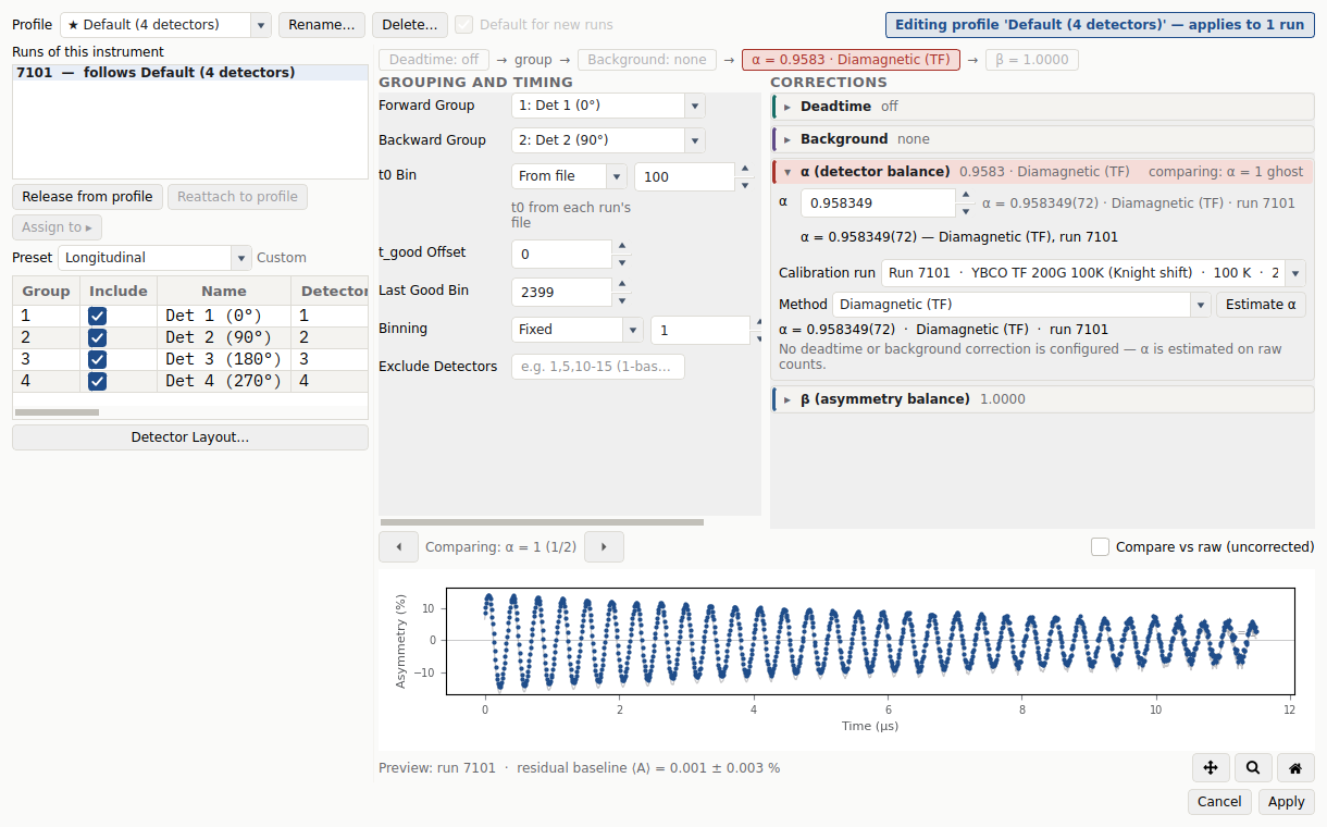
Alpha is calibrated inline, in the α (detector balance) section of the Corrections column: pick the calibration run, choose a method, and press Estimate α. The shared live preview below doubles as the before (α = 1) / after (fitted α) comparison once α is calibrated.
Alpha is calibrated inline, in the α (detector balance) section of the
Corrections column. Pick a run from the Calibration run dropdown — every run
of the current instrument is listed, with likely calibration candidates
highlighted and auto-selected: a run is flagged when its metadata carries
explicit transverse-field evidence (a structured Transverse field-geometry
classification, or a TF/wTF/transverse token in the title or
comment) and, when a field magnitude is recorded, that magnitude sits in the
weak-to-moderate window a diamagnetic calibration run conventionally occupies
(roughly 5–500 G). A run with an explicit transverse token but no recorded
field magnitude is still flagged, since the token is the stronger signal; a
field magnitude alone, with no textual evidence, is not — the value alone is
ambiguous between a weak-TF calibration run and a run whose only relation to the
window is coincidence. This heuristic only changes what is highlighted and
pre-selected: any loaded run remains choosable from the dropdown.
Choose a Method from three options:
Diamagnetic (TF) — the standard balance method for a silver or other non-relaxing transverse-field run: \(\alpha\) is fitted so the forward and backward precession signals oscillate symmetrically about zero.
General (LF/ZF) — a fit that also accommodates a genuinely relaxing or multi-component signal.
Count ratio ΣF/ΣB — the simple forward/backward integral ratio over the good-bin window (Mantid’s
AlphaCalc), with no oscillation model.
Press Estimate α. The estimate runs on a worker thread over the corrected forward/backward counts — deadtime-corrected and background-subtracted exactly as the reduction forms them — so a calibrated \(\alpha\) centres the reduced asymmetry rather than the raw totals. A note under the result reports which corrections the estimate reflected (for example “α is estimated on corrected counts (deadtime, background (range))”, or a warning when a requested correction could not be applied to the calibration run). The shared live preview doubles as the before/after comparison: once \(\alpha\) is calibrated it overlays the asymmetry at \(\alpha = 1\) against the asymmetry at the fitted \(\hat\alpha\), and reports the residual baseline \(\langle A \rangle\) so the balance is self-evident.
A successful estimate sets the profile’s alpha policy to calibrated and
records its provenance — method, source run, and uncertainty — displayed as,
for example, “α = 1.2345(67) · Diamagnetic (TF) · run 2923”. Typing a value into
the alpha field directly instead switches the policy to fixed and the
provenance to plain “manual”, since a hand-typed number no longer carries a
measurement behind it. If you change the deadtime or background settings after
calibrating, an amber banner — “α was calibrated under different
deadtime/background corrections — re-estimate so it centres the corrected
asymmetry” — flags that the calibration is stale until you re-estimate.
Per-projection alpha (WEP / vector)
A layout that exposes more than one asymmetry projection from the same
groups — GPS’s WEP FB/UD pair, EMU’s \(P_x\)/\(P_y\)/
\(P_z\) vector axes, or the transverse Top-Bottom/Fwd-Back pairs
on MuSR and HiFi — calibrates and stores \(\alpha\) per projection
rather than sharing one value. Each projection carries its own declared
alpha (GPS WEP’s FB pair defaults to musrfit’s 0.75, its UD
pair to 1.0); reducing or fitting a projection always applies that
projection’s own alpha, falling back to the profile’s base alpha only when a
projection has none declared. See Vector-polarisation mode for the EMU
per-axis alpha table and estimation buttons, which follow the same
per-projection model.
Deadtime correction
The Deadtime card of the Corrections column configures the profile’s deadtime policy inline; its header shows the live mode summary (e.g. “off”, “manual (10.000 ns avg)”) even while the card is collapsed. Four modes are available:
Offdisables the correction.Fileuses per-detector deadtime values already present in a run file. This stays the default starting point for raw histogram formats, matching WiMDA’s file-first assumption, even when the currently selected run does not itself provide file deadtime values.Manualshows a per-detector value table, editable directly, and is also where calibrated values are stored.Estimatefits the reference run’s early-time average detector rate, following WiMDA’s uniform deadtime estimate workflow, then applies that one estimated value to every detector.
The section adapts to the selected mode, showing only the controls that mode
uses so the Corrections column stays readable without scrolling. Off shows the
mode radios and a Deadtime correction is disabled. note. Manual shows
the editable Per-detector values (ns) table with its Fill all and
Cal buttons, height-capped at six rows so larger detector counts scroll
inside the table rather than the column. File and Estimate collapse to a
one-line summary — the mean deadtime value times the detector count followed by
the maximum-correction figure (for example, 10.000 ns × 4 detectors · max
correction at t=0: 1.2%) — with a Show per-detector values disclosure that
reveals the read-only table on demand; Estimate also keeps its source-run
picker and Estimate button.
The Cal button ports WiMDA’s per-detector calibration routine: it fits each detector histogram in the selected run separately, produces a resolved per-detector deadtime table, and populates the manual table with those calibrated values. The maximum correction at t=0 figure is the largest fractional correction any detector receives at the first good bin, so an unreasonable deadtime value is visible immediately rather than only showing up as a distorted asymmetry later.
When Off is selected, deadtime correction is disabled. When Estimate
is selected, the estimate is calculated from the currently selected preview
run only, then applied to every run following the profile. Cal also uses
the selected run only, but calibrates one deadtime value per detector
instead of a single shared value. The resolved deadtime values are stored on
the profile’s deadtime policy, so every run following the profile shares the
same manual, calibrated, or estimated deadtime values, just as they already
share alpha and grouping.
All modes use the same non-paralysable correction form used by musrfit
PRunBase::DeadTimeCorrection and Mantid ApplyDeadTimeCorr:
For File mode, t_dead comes from the run file when available. For
Manual, Cal, and Estimate workflows, Asymmetry resolves the
deadtime values from the profile’s policy before the correction is applied.
N_frames still comes from each dataset’s own good-frame metadata when it
is available.
PSI BIN/MDU and MusrRoot/LEM ROOT data usually do not ship NeXus-style file
deadtime constants, so File mode is commonly unavailable there. Those runs
can still use Manual or Estimate deadtime correction, with Cal
available to populate per-detector manual values from the selected preview
run. The background correction path remains separate and optional.
Background correction
The Background card of the Corrections column configures the
profile’s background policy inline for PSI-style raw histogram formats,
including PSI BIN/MDU and PSI/LEM ROOT data. This is separate from fit-model
background parameters such as A_bg: it subtracts a count background from
grouped raw forward/backward histograms before the asymmetry is calculated.
This follows musrfit’s PRunAsymmetry ordering. Histograms are first
grouped into forward and backward sums, then background is subtracted, and
then asymmetry is calculated. The section’s modes are:
None— no correction.Range— the background is estimated as the mean count in an inclusive pre-\(t_0\) bin range. If no range is given, it uses musrfit’s fallback range from0.1 * t0to0.6 * t0.Tail fit— a Poisson maximum-likelihood fit of the late-time count level, for runs where a fixed pre-\(t_0\) window is not representative.Reference run— subtracts a dedicated background run’s own grouped counts (scaled by relative good-frame count).Fixed— fixed forward/backward count values are subtracted directly.
The shared live preview below both columns always reflects the subtraction, so its effect on the asymmetry is visible as the mode changes.
For corrected histograms, Asymmetry propagates musrfit-style count
uncertainties through its standard pair formula, with alpha multiplying
the backward group.
Background subtraction can make late-time corrected forward/backward sums
very small or negative. Those bins may therefore produce asymmetries at or
beyond +/-100%. The plot keeps such low-confidence PSI points visible in
grey, matching the low-count visual treatment used for raw grouped data, and
excludes them from automatic Y-axis scaling.
The correction is off by default and disabled for ISIS/NeXus data, where deadtime correction is the file-metadata correction path. When enabled for PSI data, the applied method, estimated values, and ranges are stored on the profile’s background policy.
Comparing a correction’s effect
A pipeline strip across the top of the right pane, above both columns —
Deadtime → group → Background → α → β — makes the reduction order visible
and summarises each stage in a chip (“Deadtime: off”, “Background: tail fit”,
“α = 1.037 · Diamagnetic (TF)”, “β = 1.0000”); the group divider is a
reminder that
detector grouping, set in the Grouping and timing column, sits between deadtime
and background. Clicking a chip focuses that stage’s compare (below) and scrolls
its section into view. When a calibrated \(\alpha\) goes stale the chip
appends “ · stale” and its tooltip prompts a re-estimate. (Strictly,
\(\alpha\) and \(\beta\) are applied together in the one
asymmetry-formation step; the strip orders them for focus, not because one
precedes the other.)
Each stage wears its own identity colour — teal for deadtime, violet for background, a muted red for \(\alpha\), a steel blue for \(\beta\) — as the chip’s outline and the matching card’s header stripe, so a chip and its card read as one thing at a glance; focusing a stage’s compare fills both the chip and the card header with that stage’s soft tint.
Comparing is driven from the pipeline chips and the compare pager — there are no per-section checkboxes. Clicking a stage’s chip focuses that stage’s compare, expands its correction card, and scrolls the card into view; clicking the focused chip again clears the focus. A compound Compare vs raw (uncorrected) checkbox sits in the pager row just above the pinned preview (so it is reachable from either column). One stage is focused at a time — that keeps the two-curve plot legible — and each stage can be focused only while it has a before/after to show.
While a stage’s compare is focused, its correction card is accent-highlighted — soft accent header with an accent left edge — and the header’s right side shows what the ghost is: “comparing: without deadtime”, “comparing: without background”, “comparing: α = 1 ghost”, or “comparing: β = 1 ghost”. (The compound raw compare belongs to no single card, so it lights no card; the pager label names it.)
In the preview itself the solid curve is always the full reduction, and a dimmer ghosted curve shows the asymmetry with the focused stage removed. The ghost is named by a small inline label at its rightmost visible sample — “without deadtime”, “without background”, “α = 1”, “β = 1”, or “raw (uncorrected)” for the compound view (no deadtime, no background, \(\alpha = 1\), \(\beta = 1\)) — there is no legend, since the pager label and the highlighted card already name the comparison. The y-axis always follows the as-reduced (solid) curve alone: a ghost that sits far off-scale (an uncorrected FLAME run’s ghost can reach \(\sim 10^7\) %) never stretches the axis and never crushes the solid curve flat; the off-scale ghost’s inline label is clamped just inside the axis edge on the side it exited, so the ghost is still named. The pager label’s tooltip states the contract — “Comparing overlays one stage’s before/after — the reduction always applies every stage”: comparing never changes what Apply writes, and because the solid curve is never degraded, the residual baseline \(\langle A \rangle\) readout (shown for the \(\alpha\) compare) is always read off the fully-corrected reduction. Calibrating \(\alpha\) auto-focuses its compare, so a fresh calibration shows the balancing effect immediately; the \(\alpha\) and \(\beta\) compares are not offered in vector mode, where the per-projection \(\alpha\) table in the Corrections column owns the balance (and the scalar \(\beta\) card is hidden entirely).
The compare pager — ◀/▶ arrow buttons flanking a muted label — sits
directly above the pinned preview, below both columns, so it works regardless of
which column is focused. It drives the same shared focus
as the pipeline chips: each arrow steps through the
configured corrections in pipeline order (deadtime, background, \(\alpha\),
\(\beta\), raw), skipping any stage without a before/after to show. The label reads
“Comparing: off” when nothing is focused, and otherwise names the stage and its
position among the currently available stages, e.g. “Comparing: without
background (1/3)” or “Comparing: vs raw (3/3)”. Both arrows disable together
when no correction is configured yet. The Compare vs raw (uncorrected)
checkbox rides at the right end of the same row.
PSI Grouping
PSI BIN/MDU files use the full Grouping window, matching the interaction
model used for raw ISIS NeXus files. Initial group names and forward/backward
defaults are derived from PSI detector labels where the file provides them
(Forw/Back in BIN files, and labels such as F1/B1 in MDU
files). For PSI FLAME BIN files, filenames, detector labels, or metadata
containing FLAME select the FLAME detector layout automatically; this
includes PSI instrument strings such as LMU_BULKMUSR_FLAME. PSI HAL-9500
runs (the high-field πE3 spectrometer) are recognised from their HIFI
instrument string and tdc_hifi_* run names and open with the HAL-9500
octagonal layout; a full HAL-9500 run additionally opens already grouped into
its default Per-octant preset (see PSI HAL-9500 below), so the
angle-resolved analysis is available without opening the Grouping window. This
is a distinct instrument from the ISIS HiFi spectrometer despite the shared
hifi token. PSI GPS BIN files
(deltat_tdc_gps_* with the six Forw/Back/Up/Down/Righ/Left histograms)
select the GPS two-panel layout automatically (see PSI GPS below). This
behaviour
follows the detector metadata exposed by musrfit’s PSI raw-data reader, with
Mantid’s PSI-BIN loader used as a cross-check for BIN layout details.
When labels repeat, Asymmetry keeps one visible group per histogram and makes
the displayed names unique with numeric suffixes.
PSI data can carry a separate t0 for each detector. Asymmetry stores these
values as detector_t0_bins and aligns each detector histogram to its own
t0 before summing groups. This avoids shifting all PSI spectra through a
single global time-zero before grouping.
PSI detector names use the PSI instrument convention: Forward and
Backward are measured along the beam direction. Asymmetry’s pair-asymmetry
formula uses forward/backward relative to the initial muon spin direction.
Every PSI Longitudinal preset (GPS, FLAME, HAL-9500) now declares this
directly, in the preset itself: the Backward-named group occupies the
analysis-forward slot, so a preset used headless from the core API reduces
correctly with no GUI compensation needed. See Beam vs analysis convention
below for the physics and PSI GPS for the full per-preset listing.
ROOT Grouping
MusrRoot/LEM ROOT files also use the full Grouping window. The ROOT loader
follows musrfit’s PRunDataHandler::ReadRootFile and reads detector labels
from DetectorInfo when available, falling back to the ROOT histogram title
or hDecay name. As with PSI BIN/MDU files, repeated detector labels are
kept as separate visible groups with numeric suffixes.
ROOT files with RunInfo/Instrument set to FLAME are opened with the
FLAME detector layout available by default. If that metadata field is absent,
Asymmetry also recognises flame in the source filename. GPS MusrRoot files
(instrument LMU_BULKMUSR_GPS) expose eleven raw sub-detectors and open with
the eleven-detector GPS variant (see PSI GPS below).
ROOT DetectorInfo entries can provide detector-specific Time Zero Bin,
First Good Bin, and Last Good Bin values. Asymmetry stores these in the
grouping payload and aligns detector histograms by their own t0 before
constructing the initial asymmetry.
Detector layout editor workflow
Open Grouping from the toolbar or menu.
Click Detector Layout…
Choose instrument and preset in the right-hand panel.
Click detector sectors in the schematic to refine groups.
Apply and return to the Grouping window.
A detector can belong to multiple groups. This is required for transverse and vector-polarisation workflows.
The Grouping table includes an Include checkbox for each group. This does not change the stored detector membership of the group. Instead, it controls whether that group participates in the Individual Groups plot view and in grouped time-domain fitting.
In-app arrangement schematics
The schematic renders each detector’s full group membership, not just its primary group: a detector that belongs to more than one group — the ordinary case for transverse and vector-polarisation layouts — is drawn as several thin slices around its own segment, one colour per group it belongs to, so an overlapping arrangement such as HiFi’s manual transverse quadrants is visible directly on the schematic rather than only inferable from the group table. Hovering a detector shows its id, its physical label where the format provides one, the list of groups it belongs to (or “(none)” if ungrouped), and whether it is currently excluded. Each group’s button in the Detector Layout editor carries its live member count, e.g. “Top (18)”, and a Clear excluded button removes every detector from the exclusion set in one action, undoing exclude-mode edits without re-clicking each one.

HiFi’s Transverse (Vector) preset in the Detector Layout editor. The
boundary detectors between the Left-Right and Top-Bottom pairs belong to
two groups each, rendered as a second membership slice.
HiFi
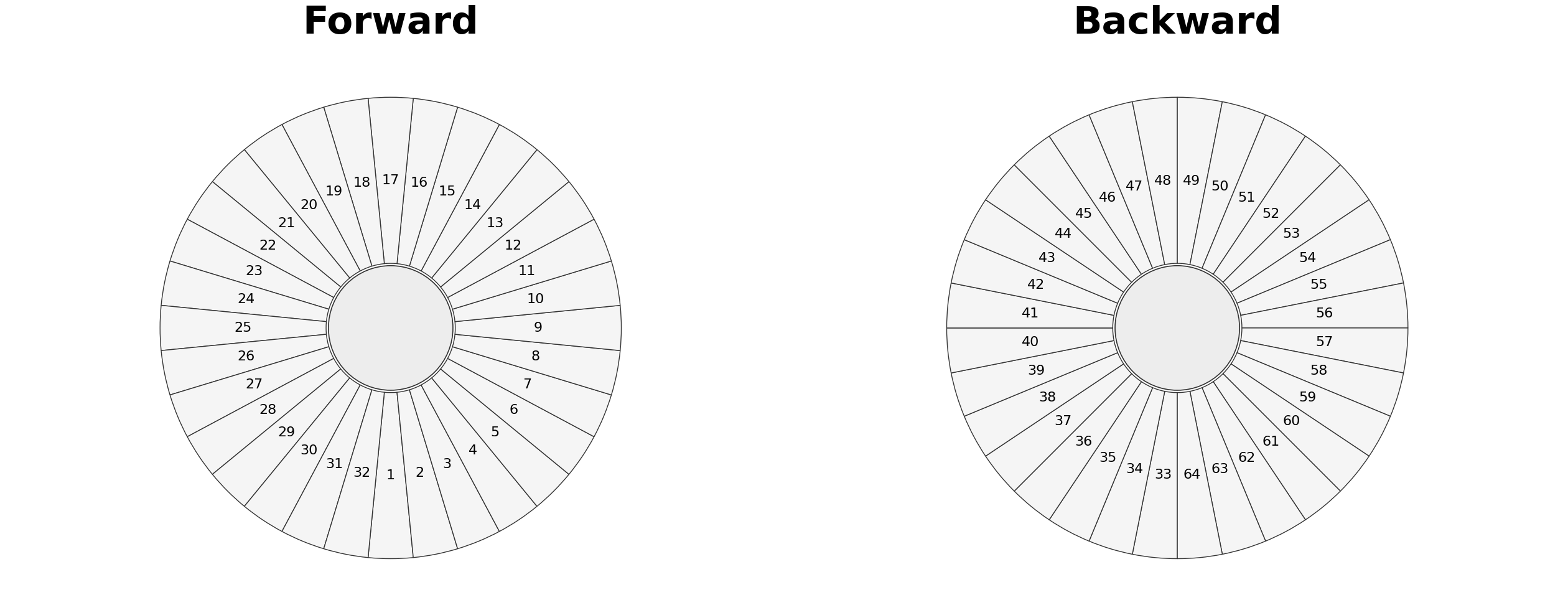
HiFi schematic matching the in-app detector arrangement.
MuSR
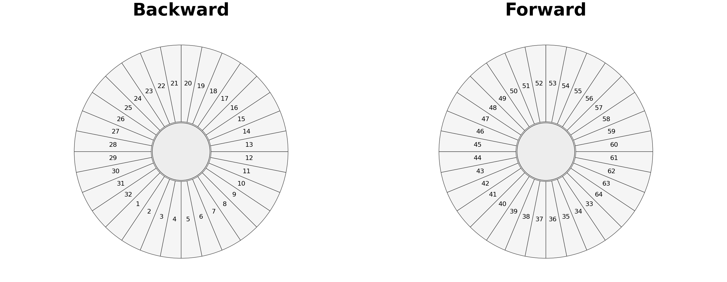
MuSR schematic matching the in-app detector arrangement.
EMU
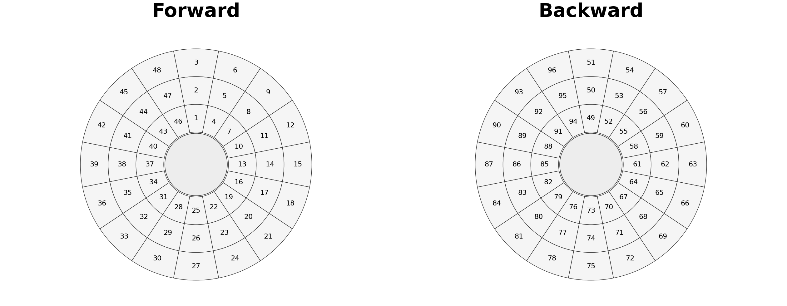
EMU schematic matching the in-app detector arrangement.
Numbering follows the EMU User Guide, Section 8.1: sector-major triplets
(inner/middle/outer ring of one sector before moving to the next sector),
sector 0 at 12 o’clock, numbers increasing clockwise looking upstream from
downstream. The three radial rings exist for stray-count rejection (Giblin
et al., Nucl. Instrum. Methods Phys. Res. A 751, 70 (2014)), not for
the Vector Polarization preset. That preset (\(P_x\)/\(P_y\)/
\(P_z\) octant composition) is an Asymmetry construct with no
facility-documented equivalent; see Vector-polarisation mode and the
module docstring in core/instrument.py::_build_emu.
PSI FLAME
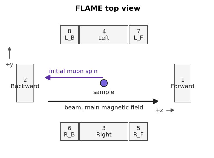
PSI FLAME top-view detector layout. The beam and main magnetic field are drawn along +z, and the initial muon spin points toward the Backward detector. FLAME detectors are rectangular plates: 1 Forward, 2 Backward, 3 Right, 4 Left, 5 R_F, 6 R_B, 7 L_F, and 8 L_B. The Left and Right banks use equal-height rectangles with the central detector drawn wider than the front/back side detectors.
PSI HAL-9500
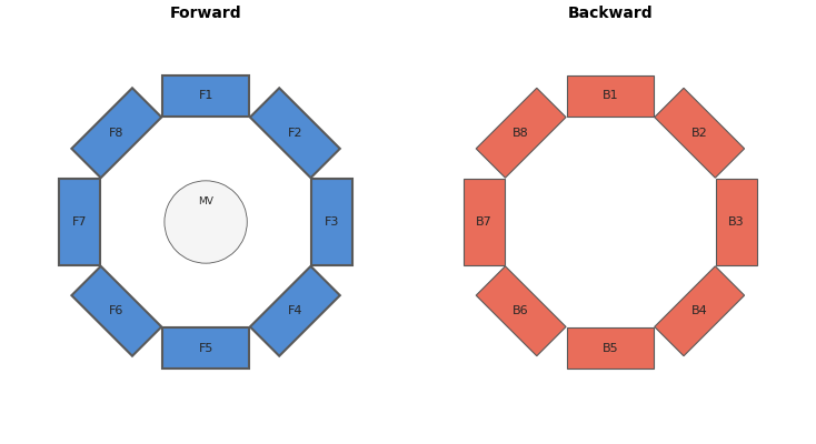
PSI HAL-9500 detector layout, viewed along the beam axis. The 16 positron
detectors form two octagonal rings of eight — a forward ring (F1–F8) and a
backward ring (B1–B8) — drawn as separate octagons. The central muon-veto
detector (MV) is shown at the centre of the forward ring. The histograms are
stored in the order MV, F1…F8, B1…B8, so detector IDs run MV → 1,
F1–F8 → 2–9, and B1–B8 → 10–17. Presets include Per-octant (default —
each azimuthal sector combining its forward and backward wedge; HAL-9500 is
a high-field spectrometer, and this is the grouping used for that work in
practice), Longitudinal (forward ring vs backward ring), and
Transverse (opposed pairs) (each forward detector as its own group,
defaulting to the F1–F5 diametric pair). A full HAL-9500 run (all 17
histograms) opens already grouped per-octant — the loader applies the
Per-octant preset automatically, so the angle-resolved per-group analysis is
available immediately without opening the Grouping window. The eight octant
groups exclude the muon-veto MV.
Some high-field .mdu runs ship only the forward ring (MV, F1…F8 —
nine histograms, no backward ring). Such a run still opens grouped
Per-octant: the preset naming backward-ring detectors (10–17) applies
over the detectors the run does contain, so each octant degrades to one
forward wedge (physically equivalent to Transverse (opposed pairs), with
the analysis pair reducing to F1 vs F5), and the absent detectors are dropped
at reduction time. This is identical to applying Per-octant by hand from the
Grouping window, where the LOG additionally notes which absent detectors were
ignored. A preset whose forward or backward analysis group is an entirely
absent ring — Longitudinal, whose backward group is the whole missing
backward ring — cannot form an asymmetry, so it is not auto-applied and the
loader’s label-based default is kept instead; applying it by hand is likewise
skipped with the missing detectors named.
PSI GPS
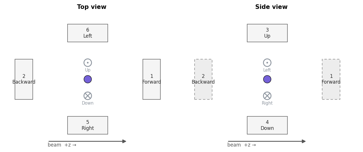
PSI GPS layout, drawn as two plan panels. The beam runs along +z toward the Forward detector. GPS surrounds the sample with six positron detectors on three orthogonal axes — Forward/Backward (beam), Up/Down (vertical) and Left/Right (horizontal-transverse) — so a single flat view cannot place all six. The Top view shows the horizontal plane (Forward/Backward and Left/Right in place; Up/Down drawn end-on, ⊙ toward you and ⊗ away); the Side view shows the vertical plane (Up/Down in place; Forward/Backward read-only; Left/Right end-on). Each detector is editable in its home panel and shown read-only for context in the other.
GPS is recognised automatically from PSI data carrying a GPS instrument
string or a deltat_tdc_gps_* run name. Two histogram conventions are
supported and presented to the user as a single “GPS” layout, selected
automatically from the histogram count — and, per Grouping profiles above,
each carries its own separate grouping profile:
the PSI-BIN export with six combined detectors (
Forw, Back, Up, Down,
Righ, Left
); andthe MusrRoot export with eleven raw sub-detectors (
Forw, Back, Up_B,
Up_F, Down_B, Down_F, Right_B, Right_F, Left_B, Left_F, Mob-RL
), where each transverse plate is split into an upstream (_B) and downstream (_F) half and a Mobile detector is added. Both variants are registered as one physical GPS instrument (the eleven-detector variant is GPS-RD internally — “ROOT sub-detectors” — but shown to the user simply as “GPS”).
Detector IDs match the histogram order in each format (detector N maps to histogram N − 1).
Note
Beam vs analysis convention. PSI names its detectors by beam direction (Forward is downstream, Backward is upstream). For surface muons the spin is antiparallel to the momentum, so the initial polarisation points toward the Backward detector. Following the GPS instrument paper (Amato et al., Rev. Sci. Instrum. 88, 093301 (2017), Eq. 2) and musrfit, the analysis convention is \(A = (B - \alpha F)/(B + \alpha F)\) — the Backward-named group occupies the analysis-forward slot. Every GPS, FLAME, and HAL-9500 Longitudinal preset declares that convention directly, while keeping the physical F/B/U/D group names, so a preset reduces correctly even when used headlessly from the core API. See Beam vs analysis convention (ISIS) below for how this differs from the ISIS naming.
Presets:
Longitudinal (default) — Forward vs Backward (analysis-forward = Backward).
Transverse (Vector) — the Up–Down and Left–Right pairs exposed as two asymmetry projections (musrfit’s
WED(L)transverse setup: UD forward = Up, RL forward = Right).Spin-rotated (B+U/F+D) — Backward+Up vs Forward+Down. When the spin rotator (a Wien filter on πM3.2) is used in transverse geometry the muon spin is rotated up by about 50°. The initial polarisation points toward Backward, so tipping it up leaves it along the Backward–Up diagonal; summing those detectors against Forward+Down realigns one asymmetry axis with the rotated spin and recovers the full amplitude. (musrfit’s own WEP phases — Backward at −45°, Up at +45° — bisect exactly along this diagonal, confirming the assignment; the
{2,3}/{1,4}detector pairing, not{1,3}/{2,4}, is the one that carries the full initial asymmetry, and the verbatim PSI header labelsForw/Back/Up/Down/Righpin detector 3 as Up.)WEP (spin-rotated) — the same rotated-spin mode following musrfit’s convention. This preset follows musrfit’s GPS instrument definition (
musredit_qt5/musrWiz/instrument_defs/instrument_def_psi.xml,<tf name="WEP">): rather than summing detectors it keeps Forward, Backward, Up and Down as four separate groups and exposes the FB and UD asymmetry pairs. The FB projection declares musrfit’s defaultalpha = 0.75and UDalpha = 1.0, and the reduction applies each projection’s own declared alpha — reducing or fitting the FB pair uses 0.75 and the UD pair uses 1.0 (see Per-projection alpha (WEP / vector) above). The per-detector phase offsets musrfit uses to encode the rotation are a fitting detail and are not stored in the layout.
The Mobile sub-detector (Mob-RL) is left ungrouped by default: it is added
to either the Right or Left detector depending on the cryostat port in use,
which the data file does not record.
Beam vs analysis convention (ISIS)
ISIS names its detector banks by the direction of the muon spin, not the beam: the bank the initial polarisation points toward is already named “Forward”, so an ISIS Longitudinal preset needs no beam-to-analysis swap — group 1 (Forward) is the analysis-forward group directly. This is the opposite naming choice from PSI (Beam vs analysis convention above), where “Forward”/”Backward” name the beam axis and the polarisation points toward the Backward-named detector instead. Asymmetry’s PSI presets absorb this difference at the preset level — declaring the Backward-named group as analysis-forward — so that the same pair-asymmetry formula, \(A = (F - \alpha B)/(F + \alpha B)\) read with each instrument’s own analysis-forward group, is correct for both naming conventions without a per-instrument special case anywhere downstream of the grouping payload.
A classic PSI GPS PSI-BIN file stores only five histograms — Forward, Backward, Up, Down, and Right, with no Left counter recorded. The Transverse preset’s Left group is then simply empty for that run; grouping, calibration, and reduction all handle an empty group gracefully (an empty forward or backward group falls back rather than dividing by zero), so an older GPS file loads and analyses normally, just without a usable Left-Right projection.
FLAME, HAL-9500, and GPS-RD detector labels (R_F, L_B, and similar)
come from the data file’s own metadata rather than a published facility
table — the facility user guides document detector numbering, not these
compact label strings — so Asymmetry’s schematic and group names follow
whatever the file itself records.