Temperature scan through a magnetic transition

This chapter is a worked example showing how Asymmetry handles a zero-field (ZF) μSR temperature scan through a magnetic ordering transition. It runs on the real muon-school EuO dataset — the PSI GPS histograms deltat_pta_gps_2923–2973 — which is the same data analysed by Blundell et al. in their study of the localised ferromagnet EuO (Phys. Rev. B 81, 092407 (2010)). Every number and figure below comes from driving the GUI over those files, so the results can be checked directly against the paper. The same workflow applies, with minor adaptations, to metallic ferromagnets and to molecular antiferromagnets; two such variants are shown at the end.

EuO is a textbook case. It is a ferromagnetic semiconductor in which the Eu²⁺ 4f⁷ moments are nearly fully localised, making it one of the best physical approximations to a Heisenberg ferromagnet, and it orders at a conveniently accessible Curie temperature \(T_C \approx 69\) K. The zero-field muon therefore precesses in a clean spontaneous internal field whose collapse toward \(T_C\) traces out the magnetic order parameter.

Physical motivation

A muon stopped in an ordered magnetic phase sees a static local field \(B_\mu\) set by the dipolar and contact (hyperfine) contributions of the surrounding ions. Its spin precesses at the Larmor frequency

\[\nu_\mu = \frac{\gamma_\mu}{2\pi}\, B_\mu ,\]

where \(\gamma_\mu / 2\pi = 135.5\;\mathrm{MHz\,T^{-1}}\). As temperature rises toward \(T_C\) the sublattice magnetisation falls — and so does \(B_\mu\) — until the precession washes out entirely and the signal reverts to a slow paramagnetic relaxation. The frequency \(\nu(T)\) is thus a direct measure of the magnetic order parameter. Near \(T_C\) it follows a power law

\[\nu(T) = \nu_0 \left(1 - \frac{T}{T_C}\right)^{\beta},\]

with the critical exponent \(\beta\) depending on the universality class (\(\beta = 1/2\) in Landau mean field, \(\beta \approx 0.37\) in the 3D Heisenberg model, \(\beta \approx 0.33\) in 3D Ising). Measuring \(\beta\) from μSR is one of the most direct ways to test which class a given material belongs to — but, as EuO illustrates below, the exponent recovered depends critically on the temperature range fitted.

The data

The zero-field temperature scan is runs 2923–2960 (the file series continues to 2973 with a set of transverse-field 60 G runs, not used here). The muon-school folder ships a logbook giving the measured sample temperature of each run; the scan reads from \(T = 1.6\) K, deep in the ordered phase, up through \(T_C \approx 69\) K into the paramagnet at 200 K. Two early runs (2923, 2924) are dropped because their short statistics and unreliable thermometry make their temperatures untrustworthy, and the very-near-\(T_C\) runs, where the precession is barely a fraction of a cycle before it damps away, are left out of the order-parameter trend. That leaves eighteen well-resolved ZF runs from 1.6 K to 68.7 K.

Asymmetry reads the PSI .bin histograms natively, so no format conversion is needed — Open the run series and the temperatures and fields populate the browser directly from the file headers.

Step 1 — Load and inspect

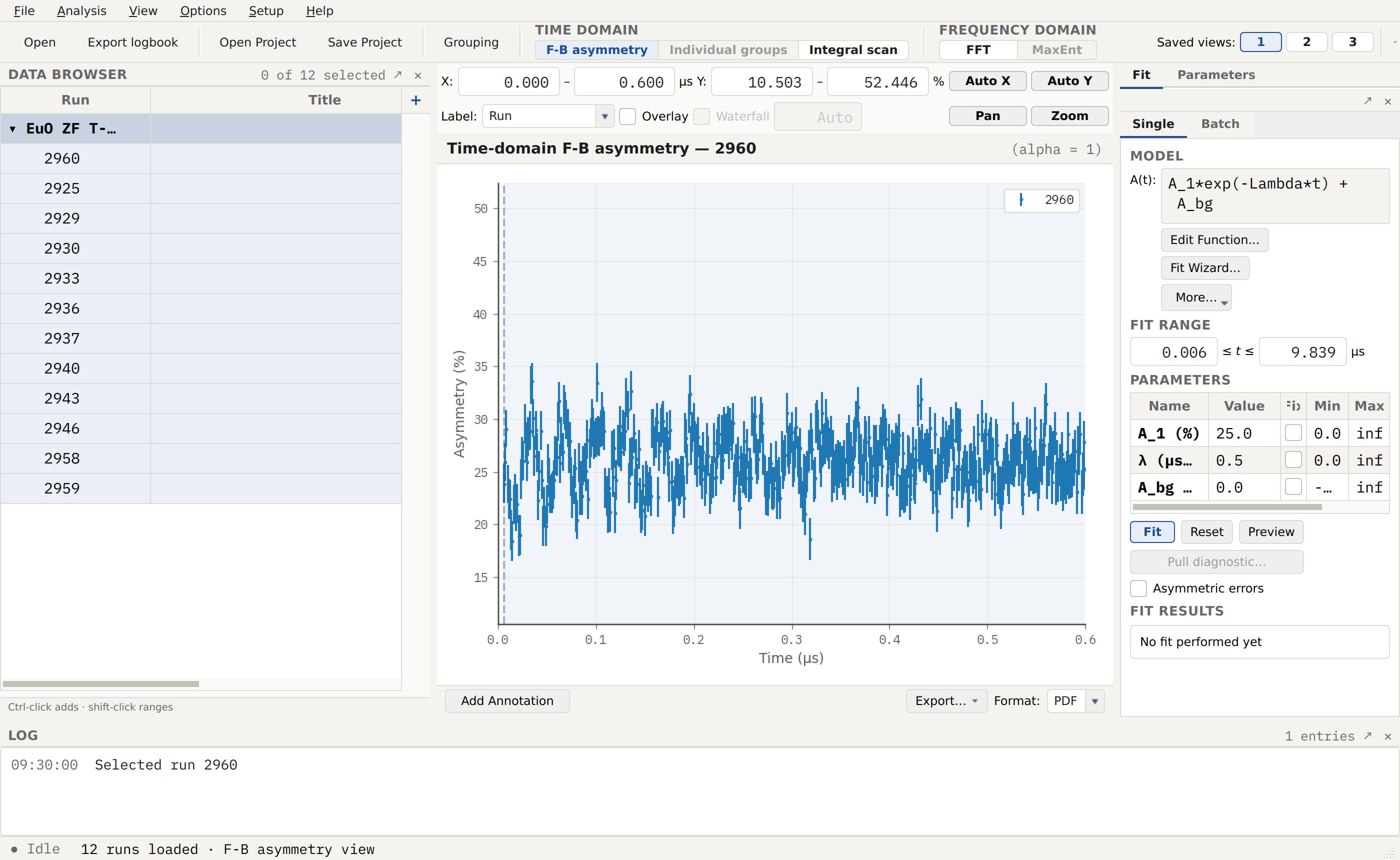
The zero-field EuO scan loaded from the real deltat_pta_gps histograms. The data browser lists one run per temperature, sorted coldest-to-hottest; the plot shows the base-temperature run (2960, 1.6 K) over its first 0.6 μs, where the spontaneous precession is fastest. The T (K) column is read straight from the file metadata, and every run is zero-field (B (G) = 0). The PSI headers carry no run title, so the Title column is blank — cosmetic, and harmless.

The data browser doubles as a run logbook: with the runs grouped and sorted by temperature, the scan reads top-to-bottom for the rest of the workflow. Selecting the base-temperature run and zooming into the first fraction of a microsecond already shows a coherent oscillation — the qualitative signature that the sample is magnetically ordered. Clicking up through the runs shows the precession slow and damp as the transition is approached, and disappear entirely above \(T_C\). This visual inspection is the first half of model selection: it is already clear that an oscillatory model is needed below \(T_C\) and a plain relaxation above it.

Step 2 — Group consistently across the scan

The zero-field spontaneous precession is carried by the transverse Forward/Backward detector pair, and Asymmetry’s loader picks that pair by default for these GPS files, so the F-B asymmetry representation shows the oscillation with no manual grouping. The forward–backward asymmetry is formed as

\[G_z(t) = \frac{N_f(t) - \alpha\, N_b(t)}{N_f(t) + \alpha\, N_b(t)} ,\]

with \(\alpha\) the detector-balance constant. Here \(\alpha\) is left at its uncalibrated value of 1, which leaves the asymmetry sitting on a large (~28 %) constant offset from the unequal detector efficiencies. That offset is harmless — it is absorbed by an additive constant term in the fit model (Step 3) — but it dominates the vertical scale, so the time-domain plots below are zoomed in time and framed to the oscillation window. When a balanced asymmetry is wanted, open the Grouping dialog, use Calibrate… to estimate \(\alpha\) from a transverse-field run, and Apply the grouping to the whole selection so every run in the scan is treated identically.

Step 3 — Fit an ordered run

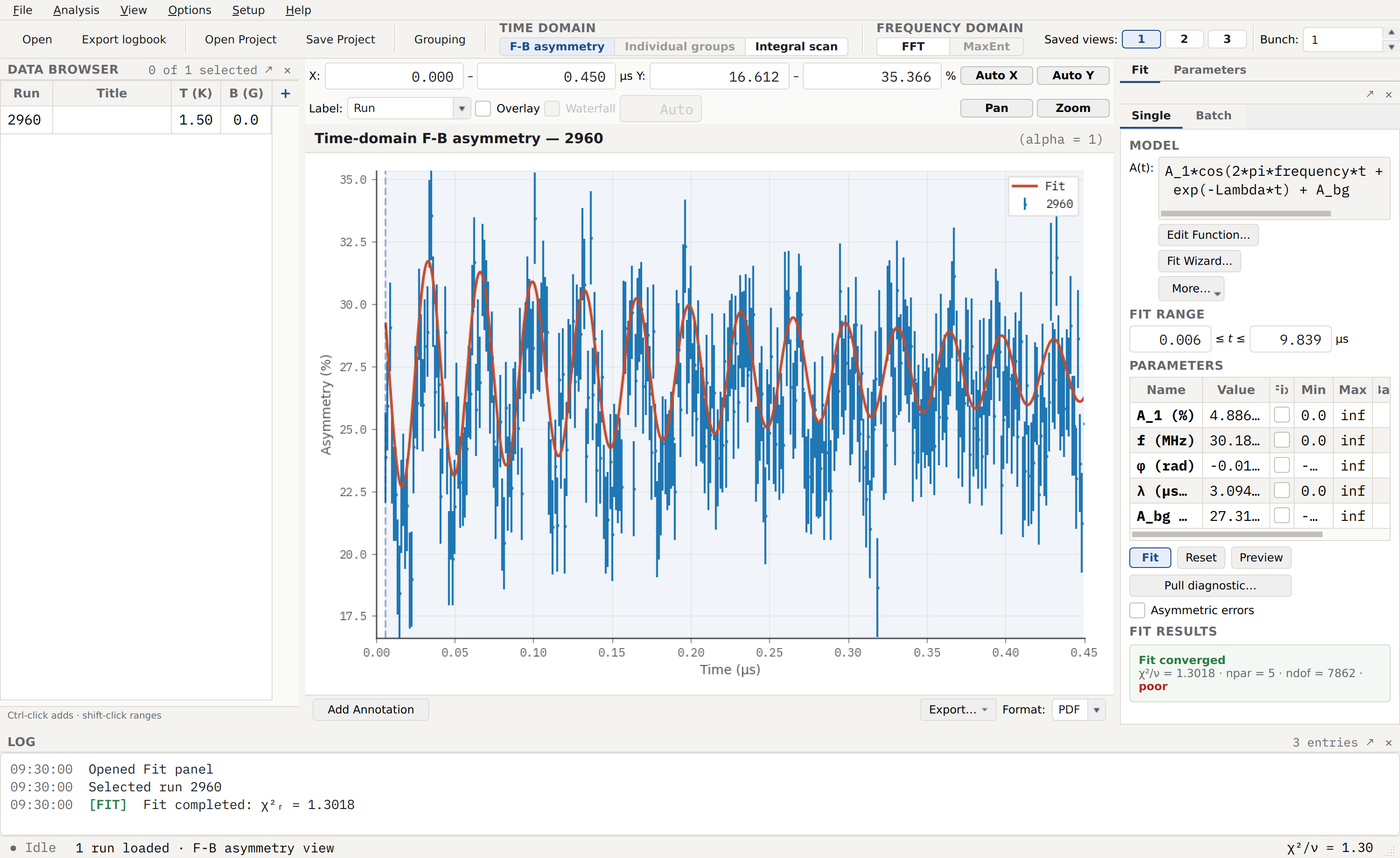
The converged single-run fit on the base-temperature run (2960, 1.6 K), zoomed to the first 0.45 μs so the individual cycles resolve. The model is Oscillatory * Exponential + Constant — a damped cosine on a constant background — and the parameter table reports \(f = 30.18\;\mathrm{MHz}\), a damping rate \(\lambda = 3.09\;\mathrm{\mu s^{-1}}\), and the large \(A_{bg} = 27.3\,\%\) baseline that the uncalibrated \(\alpha\) leaves behind. The reduced chi-square is \(\chi^2_\nu = 1.30\).

For each ordered run the fit model is a single damped cosine on a constant background,

\[A(t) = A_1 \cos(2\pi\, f\, t + \varphi)\, e^{-\lambda t} + A_{bg},\]

entered as the composite Oscillatory * Exponential + Constant. The frequency at base temperature, \(f = 30.18\;\mathrm{MHz}\), reproduces the paper’s \(\nu(0) \approx 30\) MHz and corresponds to an internal field \(B_\mu(0) = f/(\gamma_\mu/2\pi) = 0.22\;\mathrm{T}\) at the muon site.

One practical point governs the whole scan: seed the frequency near the expected value and warm-start it downward as the temperature climbs. The single-frequency fit has a spurious low-amplitude minimum, and a seed that starts too far below the true frequency collapses into it. Fitting in ascending-temperature order, carrying each converged \(f\) forward as the seed for the next run, keeps every fit in the correct minimum. The Fit Wizard… can be used on a mid-transition run to confirm the model choice before committing to the batch; below \(T_C\) it settles on the damped-oscillation family, above \(T_C\) on a plain exponential.

The frequency-domain view gives an independent check that only one precession frequency is present:

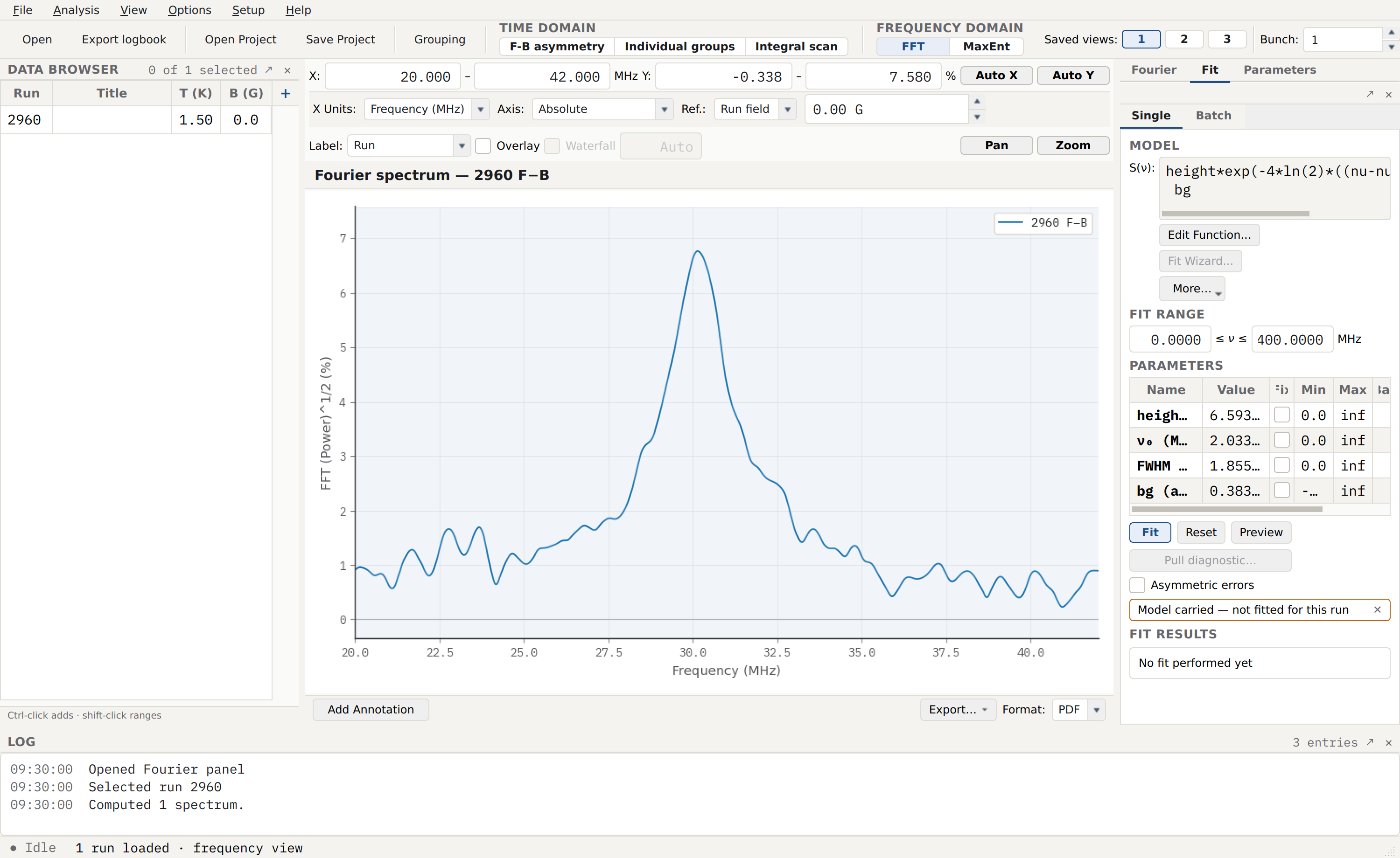
The FFT of the base-temperature run over the Forward/Back pair, with a Lorentzian Apodisation matched to the signal’s short coherence time. A single precession line stands clear at \(\nu \approx 30\;\mathrm{MHz}\), confirming that EuO orders with a single muon site and a single internal field — the frequency-domain analogue of Blundell et al. Fig. 1(c). The averaged grouped transform carries a low-frequency skirt from the detector baselines, so the view is framed to 20–42 MHz where the line dominates.

The qualitative collapse of the order parameter is seen most vividly by overlaying several runs across the transition:

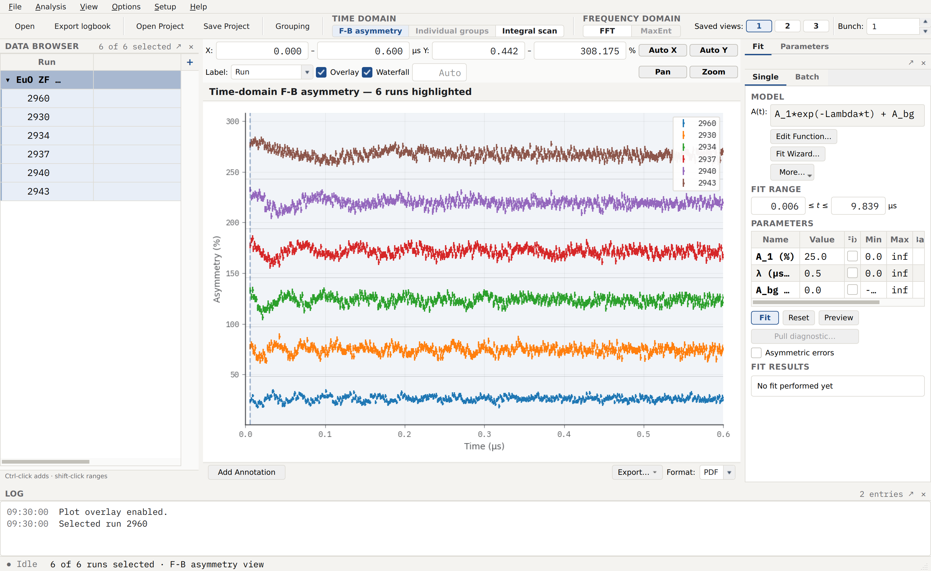
A waterfall of six zero-field spectra from 1.6 K (bottom) to 68.3 K (top). The precession visibly slows as \(\nu(T)\) falls toward \(T_C\): the base-temperature trace fits many cycles into the first 0.6 μs, while the hottest trace barely completes one before it damps away. This is the order-parameter collapse read straight off the raw time-domain data, before any trend fit.

Step 4 — Trend the order parameter

Repeating the single-run fit across the scan yields one frequency per temperature. Opening the Fit Parameters panel (from the Analysis menu) and selecting all the runs populates a trend table; choosing f (MHz) for the y-axis plots the order parameter against temperature.

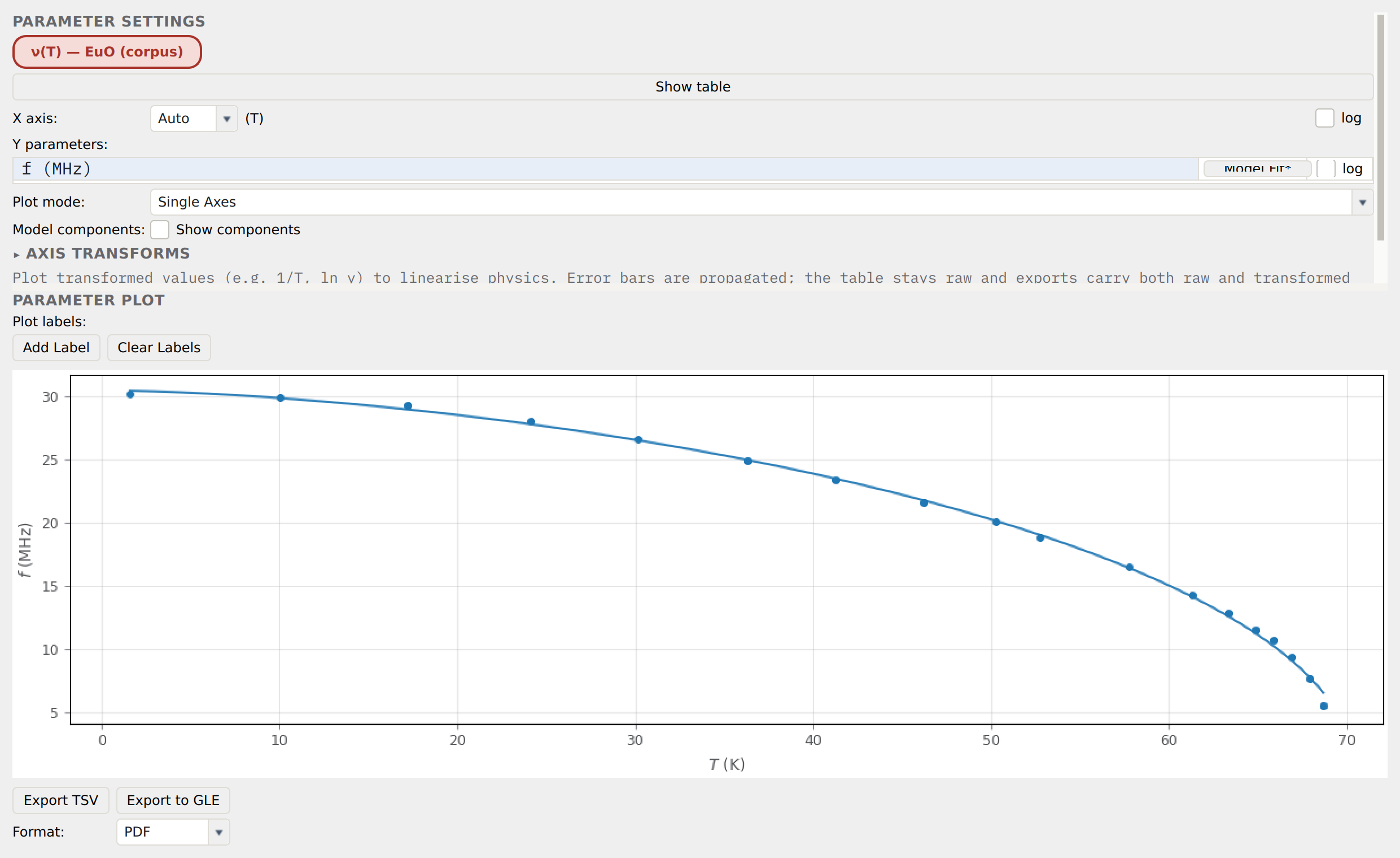
The EuO order parameter: the spontaneous zero-field precession frequency \(\nu(T)\) from eighteen real per-run fits (1.6 → 68.7 K), with the fitted OrderParameter power law overlaid (the Model Fit* button flags the active fit). The frequency starts at \(\sim 30\;\mathrm{MHz}\) at base temperature and falls with downward concavity toward zero at \(T_C \approx 69\;\mathrm{K}\). The fitted curve reproduces the paper’s Fig. 1(d) — but see the caveat below on which exponent it does, and does not, measure.

Step 5 — Fit the order parameter to a power law

In the trend panel, click Model Fit on the f (MHz) row and fit the built-in OrderParameter model,

\[\nu(T) = \nu_0 \left[1 - (T/T_C)^{\alpha}\right]^{\beta}, \quad T < T_C ,\]

which is the phenomenological form used in the paper and reduces to the Landau power law \(\nu_0 (1 - T/T_C)^{\beta}\) when \(\alpha = 1\). The model vanishes identically at and above \(T_C\), so the temperature at which \(\nu\) reaches zero constrains \(T_C\) directly.

Fitting the full 1.6–68.7 K range recovers \(\nu_0 \approx 30.6\;\mathrm{MHz}\), \(\alpha \approx 1.5\), \(\beta \approx 0.44\), and \(T_C \approx 69.9\;\mathrm{K}\). These match the paper’s own full-range phenomenological numbers (\(\alpha \approx 1.5\), \(\beta \approx 0.4\)), and the amplitude \(\nu_0 \approx 30\;\mathrm{MHz}\) and \(T_C\) near 69 K are both sound. But the exponent from this fit is not the reliable critical \(\beta\).

Critical versus phenomenological exponents — a teachable trap

The full-range fit reproduces the paper’s phenomenological curve, but Blundell et al. explicitly warn that its exponent (\(\beta \approx 0.4\)) is not the critical exponent. The authoritative value, \(\beta = 0.32(1)\) with \(T_C = 69.05(1)\;\mathrm{K}\), comes from a separate fit restricted to the critical regime — small \(1 - T/T_C\), on log–log axes (the paper’s Fig. 3) — which the whole-curve fit does not perform. The whole-curve fit also runs \(T_C\) a little high (\(\approx 69.9\) versus 69.05 K) because \(\nu\) has not quite reached zero at the last included run. So the trend render above is correct as a full-range order-parameter fit, but recovering the published critical \(\beta\) requires the log–log restriction. This regime sensitivity is a genuine physics lesson, not a quirk of the program: the exponent you extract depends on how close to \(T_C\) you dare to fit.

Reproducing the trend fit outside the GUI

The trend can be exported (Export TSV) and refitted with scipy.optimize.curve_fit. Using the per-run frequencies from the scan:

import numpy as np
from scipy.optimize import curve_fit

# Per-run ZF fit results (measured sample T, fitted frequency)
T = np.array([1.6, 10.1, 17.2, 24.2, 30.1, 36.3, 41.3, 46.2,
              50.3, 52.8, 57.8, 61.3, 65.9, 68.7])
nu = np.array([30.19, 29.86, 29.22, 27.98, 26.61, 24.88, 23.41,
               21.58, 20.06, 18.79, 16.46, 14.24, 10.66, 5.53])
nu_err = np.full_like(T, 0.3)

def order_parameter(T, nu0, Tc, alpha, beta):
    arg = np.clip(1.0 - (T / Tc) ** alpha, 1e-9, None)
    return nu0 * arg ** beta

popt, _ = curve_fit(order_parameter, T, nu, sigma=nu_err,
                    p0=[30.0, 69.0, 1.5, 0.4])
nu0, Tc, alpha, beta = popt
print(f"nu0 = {nu0:.1f} MHz, Tc = {Tc:.1f} K, "
      f"alpha = {alpha:.2f}, beta = {beta:.2f}")

This returns the full-range phenomenological numbers (\(\alpha \approx 1.5\), \(\beta \approx 0.4\)); restricting the arrays to the runs nearest \(T_C\) and fitting \(\log \nu\) against \(\log(1 - T/T_C)\) is what recovers the critical \(\beta = 0.32(1)\).

Interpretation

The analysis pins down several physical quantities:

• \(T_C \approx 69\) K is the Curie temperature; the critical-regime fit sharpens it to \(69.05(1)\) K.

• \(\beta = 0.32(1)\) (critical regime) places EuO near the 3D Heisenberg / Ising boundary, consistent with a nearly isotropic localised-moment ferromagnet.

• \(\nu_0 \approx 30\;\mathrm{MHz}\) gives the muon-site internal field \(B_\mu(0) \approx 0.22\;\mathrm{T}\). In EuO the muon sits at the ¼¼¼ interstitial site where the dipolar field vanishes, so this field is dominated by the hyperfine (contact) contribution — combined with a dipolar-tensor calculation it fixes both the site and the hyperfine coupling.

• The damping \(\lambda(T)\) rises toward \(T_C\), the signature of critical slowing-down of the spin fluctuations.

A more accurate \(\beta\) would need more temperature points within a few kelvin of \(T_C\), a consistent grouping across every run, and asymmetric error analysis on the per-run fits.

Variants

The same load → group → per-run fit → trend workflow carries over to other magnets; two contrasting cases from the muon-school corpus show its range.

Ferromagnetic nickel — a metallic ferromagnet

Nickel is a 3D Heisenberg ferromagnet with \(T_C \approx 631\) K, and the muon precesses in its spontaneous internal field with no applied field at all — the cleanest possible demonstration that the signal is intrinsic to the ordered state.

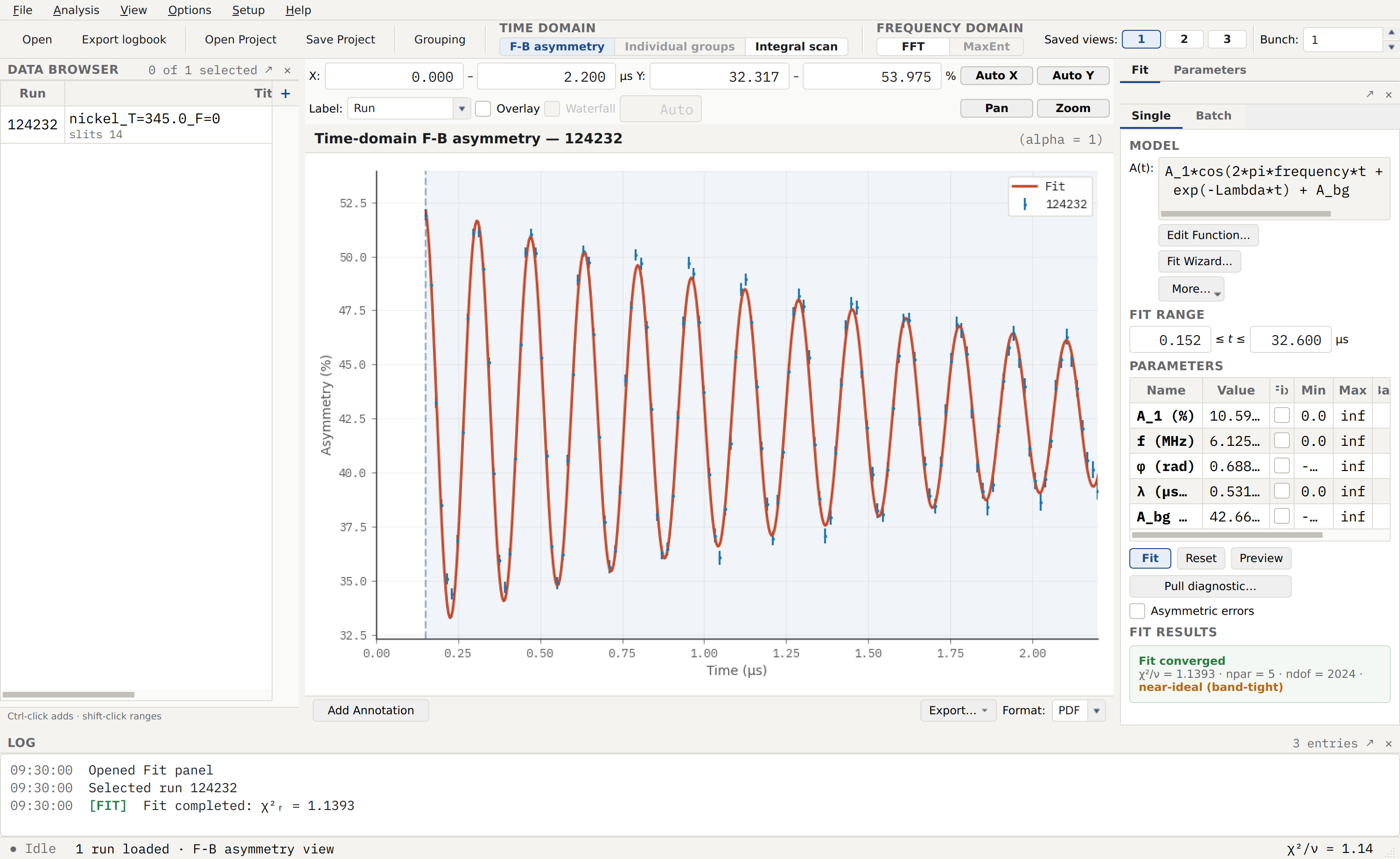
Spontaneous zero-field precession in nickel at 618 K (\(0.98\,T_C\)), from the EMU/ISIS run 124232, fitted with the same Oscillatory * Exponential + Constant model: \(f = 6.13\;\mathrm{MHz}\) (\(B_\mu \approx 0.045\;\mathrm{T}\)), \(\chi^2_\nu = 1.14\). Note the run label reads T=345 — see the metadata caution below.

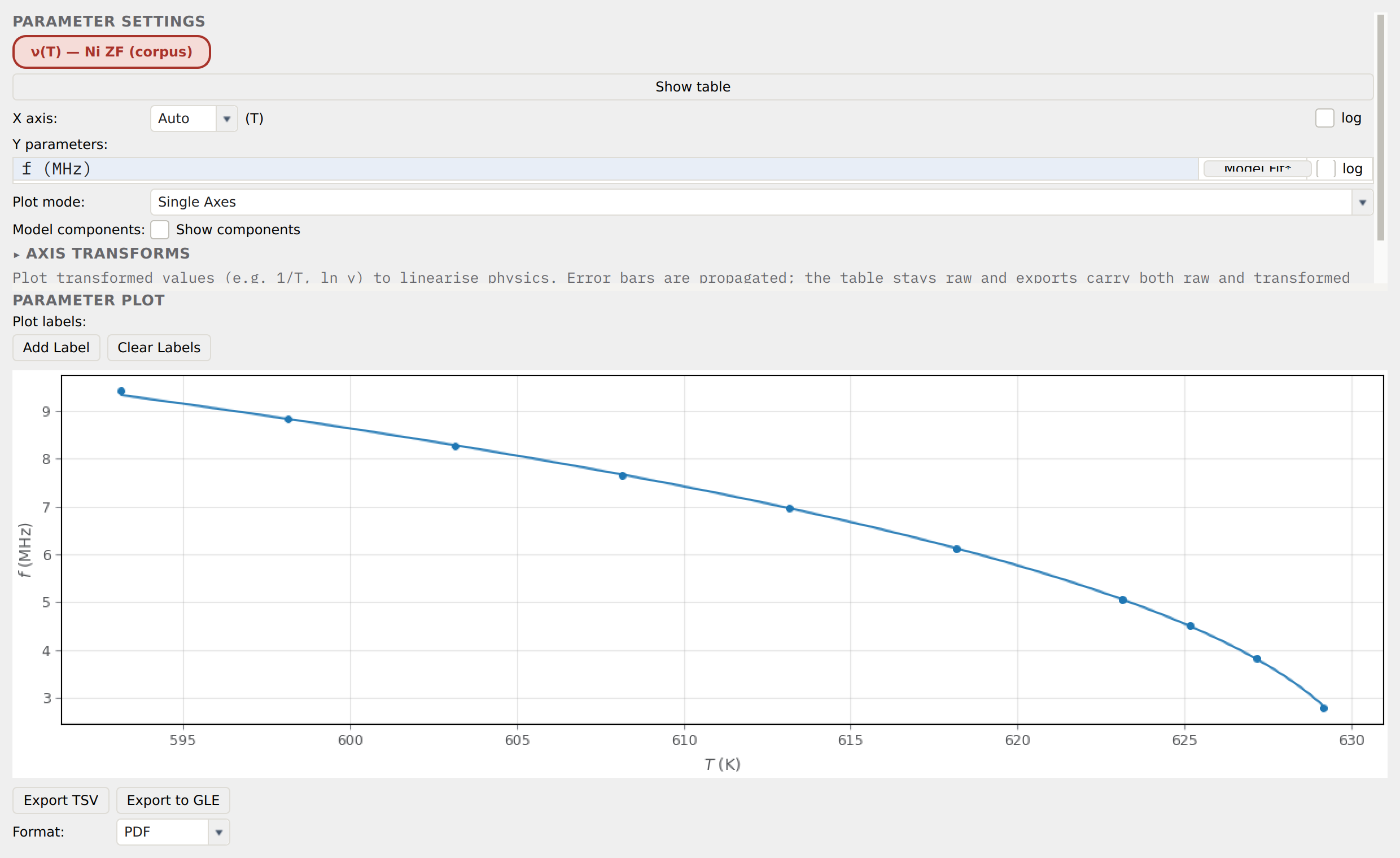
The nickel order parameter over 593–629 K, fitted with the OrderParameter law (\(\alpha\) fixed at 1, matching the \(f_{ZF}(T) \propto (T_C - T)^{\beta}\) form). The fit returns \(T_C = 630.9(2)\;\mathrm{K}\) — exactly the literature Curie temperature — and \(\beta = 0.390(8)\), close to the 3D Heisenberg value (0.367) and clearly distinct from mean-field (0.5) and 3D Ising (0.326), the expected class for bulk nickel.

Metadata vigilance — these temperatures are in °C

The nickel run labels and the on-file temperatures are the furnace controller’s Celsius readings, even though the file’s units attribute claims kelvin. The 618 K run above is labelled T=345 (i.e. 345 °C). Read naively as kelvin, the scan would place \(T_C\) near 358 K and disagree with the literature by a factor of almost two; converting to kelvin (\(+273.15\)) makes \(345\,^{\circ}\mathrm{C} = 618\;\mathrm{K}\) and \(358\,^{\circ}\mathrm{C} = 631\;\mathrm{K}\), the known \(T_C\), and every consistency check falls into place. Always confirm what a temperature axis actually means before trusting a transition temperature read off it — the critical exponent is unaffected by the offset (it cancels in \(T_C - T\)), but \(T_C\) itself is not.

A molecular antiferromagnet — the low-frequency contrast

Where EuO precesses at 30 MHz and nickel at a few MHz, a molecular antiferromagnet orders in a far weaker internal field and precesses more slowly still — a useful reminder that the same model spans three orders of magnitude in frequency.

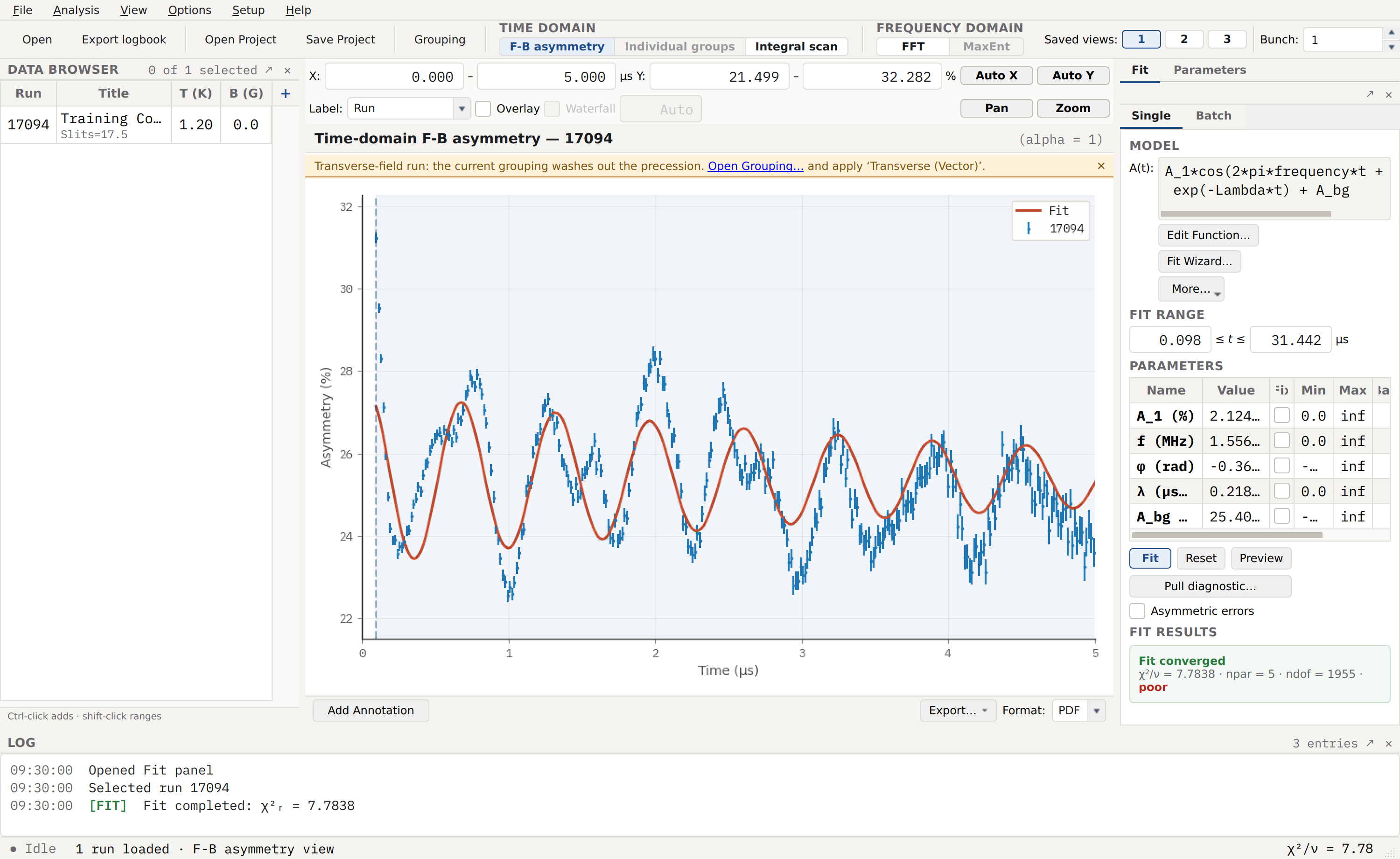
The base-temperature (1.2 K) zero-field run of a molecular antiferromagnet from the MUSR/ISIS corpus, fitted with the same composite model: \(f = 1.56\;\mathrm{MHz}\), a period of ~0.65 μs that is visible cycle-by-cycle over several microseconds. The fine 16 ns time base and low per-run statistics give a high \(\chi^2_\nu\), but the fit tracks the oscillation and the frequency is what matters.

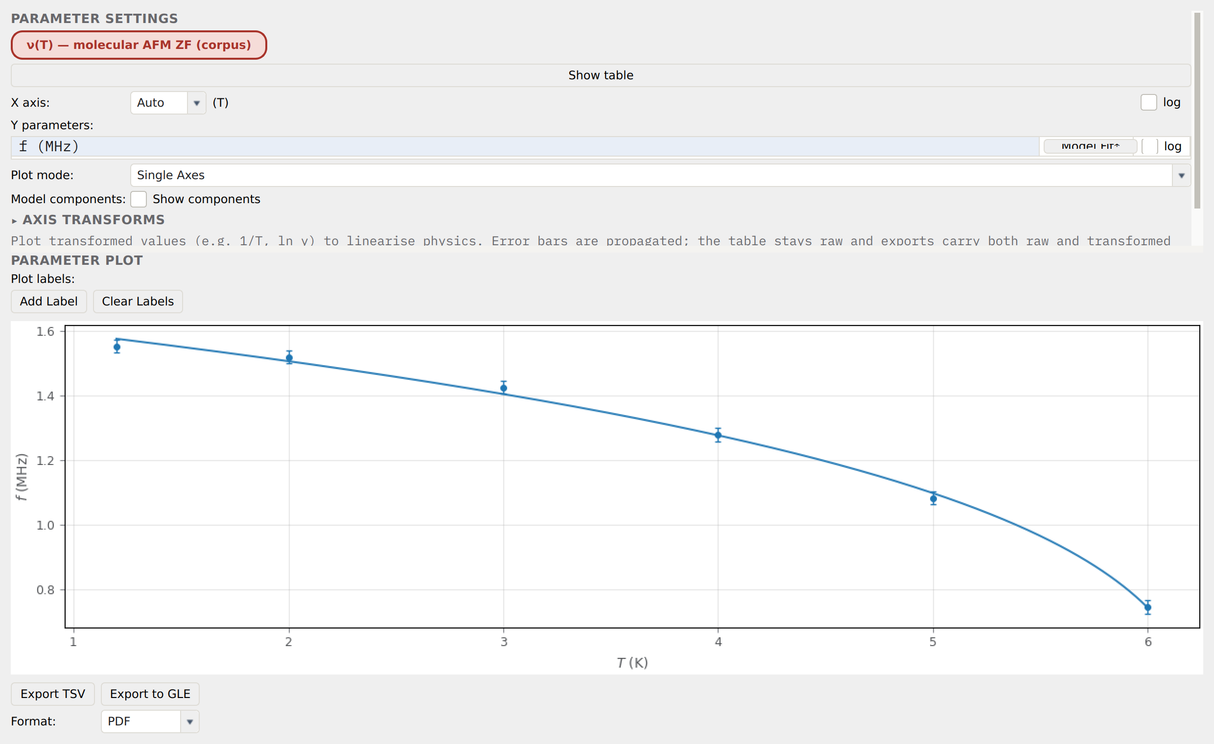
The order parameter for the molecular antiferromagnet: \(\nu(T)\) falls from 1.56 MHz at 1.2 K toward zero between 6 and 7 K, giving a Néel temperature \(T_N \approx 6.3\;\mathrm{K}\) from the OrderParameter fit — consistent with a direct comparison of the 6 K (still oscillating) and 7 K (paramagnetic) spectra. With only six points, three of them on the flat low-temperature plateau, the exponent is loosely constrained and is not quoted as a result; \(T_N\) is the robust deliverable here.

Common pitfalls

• One composite model across all temperatures. The change of regime at \(T_C\) means a single model — always oscillatory, say — will silently underweight the paramagnetic runs. Use an oscillatory model below \(T_C\) and a plain relaxation above it.

• A cold frequency seed. The single-frequency fit has a spurious low-amplitude minimum. Seed the frequency near the expected value and warm-start it downward through ascending temperature, so no run collapses into the wrong minimum.

• Reading the exponent from the whole curve. The full-range phenomenological fit is not a critical-exponent measurement. Restrict to the near-\(T_C\) regime on log–log axes for the reliable \(\beta\).

• Trusting a temperature axis blindly. As the nickel example shows, file metadata can be in the wrong units. Confirm what the temperature means before quoting a \(T_C\).

References

References

• S. J. Blundell, T. Lancaster, F. L. Pratt, P. J. Baker, W. Hayes, J.-P. Ansermet, and A. Comment, Phys. Rev. B 81, 092407 (2010). The EuO dataset analysed here; the order parameter is Fig. 1(d) and the critical-regime fit (\(\beta = 0.32(1)\), \(T_C = 69.05(1)\) K) is Fig. 3.

• M. L. G. Foy, N. Heiman, W. J. Kossler, and C. E. Stronach, Phys. Rev. Lett. 30, 1064 (1973). The nickel spontaneous-precession measurement (\(T_C = 630\) K, saturation internal field).

• S. J. Blundell, R. De Renzi, T. Lancaster, and F. L. Pratt, Muon Spectroscopy: An Introduction (Oxford University Press, Oxford, 2022), Ch. 6.1–6.2 (magnetism, Landau theory, and critical exponents).

• A. Amato and E. Morenzoni, Introduction to Muon Spin Spectroscopy: Applications to Solid State and Material Sciences, Lecture Notes in Physics Vol. 961 (Springer, Cham, 2024), Ch. 5 (μSR in ordered magnets, antiferromagnets, and unconventional order parameters).

• T. Lancaster et al., Phys. Rev. B 75, 094421 (2007). A real-data example on a molecular magnet with several precession frequencies near \(T_C\).

Cross-references

• Loading Data — load formats, including PSI .bin.

• Detector Grouping and Layout — group definitions and α calibration.

• Fit wizard — the model-recommendation tool.

• Parameter trending — the trend panel.

• Composite models — combining oscillatory and relaxation envelopes.