Superconductor penetration depth from σ(T)
This chapter is a worked example of the canonical superconductor μSR
workflow: extract the temperature dependence of the vortex-lattice
depolarisation rate \(\sigma(T)\) from transverse-field (TF) μSR data
in the mixed state, convert it to the magnetic penetration depth
\(\lambda_L\), and read the pairing physics from the shape of the
curve. The data are real. They come from the A high-Tc cuprate example
of the WiMDA muon-school corpus — a bismuth-strontium-calcium-copper-oxide
(BiSCCO, Bi-2212) sample measured on the ISIS MUSR spectrometer at
400 G and 200 G transverse field over 10–125 K. Every screenshot below is
generated by driving Asymmetry over the corpus .nxs runs, and every
fitted number is graded against the reference WiMDA .fit/.dat
outputs shipped with that example.
The same workflow reappears, with material-specific twists, in two further corpus examples cross-referenced at the end: the iron-pnictide LiFeAs, where the linewidth is reported as a field width \(B_\mathrm{rms}(T)\), and the noncentrosymmetric superconductor Re₆Zr, where the TF superfluid density sits alongside a zero-field time-reversal-symmetry-breaking signal.
Physical motivation
In the vortex state of a type-II superconductor, between \(H_{c1}\) and \(H_{c2}\), an applied transverse field penetrates the sample as a lattice of flux tubes. A muon stops at a random position relative to that lattice and samples the inhomogeneous internal field, drawn from the lattice’s field distribution \(p(B)\). The distribution is asymmetric: a sharp peak at the saddle-point field between three vortices, with a long tail toward the high-field cores (see Brandt, Phys. Rev. B 37, 2349 (1988)). The TF-μSR line is well approximated by a Gaussian relaxation of the time-domain asymmetry,
whose second moment is set by the width of \(p(B)\), \(\sigma = \gamma_\mu \langle \Delta B^2 \rangle^{1/2}\), with \(\gamma_\mu / 2\pi = 135.5\;\mathrm{MHz/T}\). For a triangular vortex lattice in the London limit \(\sigma\) is fixed by the penetration depth alone, so a single measured number returns \(\lambda_L\). The WiMDA teaching example uses the compact guide relation
so that \(\lambda_L = \sqrt{75780/\sigma}\).
The temperature dependence carries the physics. The superfluid density \(\rho_s(T) \propto \sigma(T) \propto 1/\lambda^2(T)\) reflects the superconducting gap structure: a single isotropic s-wave gap freezes \(\rho_s(T)\) exponentially as \(T \to 0\); a d-wave gap with line nodes gives a linear-in-\(T\) decrease at low \(T\); a two-gap (s+s) system shows a shoulder marking the smaller gap’s freezing scale.
Derivation — the London-limit σ ↔ λ relation and its conventions
For an ideal triangular flux-line lattice deep in the mixed state (\(H_{c1} \ll B \ll H_{c2}\), \(\lambda \gg \xi\)) the second moment of \(p(B)\) reduces to the Brandt form
with \(\Phi_0\) the flux quantum. Asymmetry implements this as
asymmetry.core.fitting.sc.constants.sigma_to_lambda_nm(), using
\(\gamma_\mu\) in rad s⁻¹ T⁻¹. The teaching guide’s coefficient
(75780, with \(\sigma\) in μs⁻¹ and \(\lambda\) in nm) and
Bernhard et al.’s equivalent \(\sigma = 7.086\times10^{4}\,
\lambda_{ab}^{-2}\) (Phys. Rev. B 52, 10488 (1995)) differ by about
7 %: they are the same Brandt relation written in different conventions.
The absolute \(\lambda_L\) therefore carries a convention-level
ambiguity of order 10 %, while the shape of \(\lambda_L(T)\) — flat
at low \(T\), divergent near \(T_c\) — is convention-independent
and is what fixes the gap structure.
The data
The A high-Tc cuprate example ships 48 ISIS muon runs. The authoritative deliverable is the MUSR 400 G temperature scan (runs 1276–1289, 10–125 K), a single Gaussian-relaxed precession fitted run by run to give \(\sigma(T)\); a companion MUSR 200 G scan (runs 1290–1303) supports the field comparison, and an EMU 150 G scan is present but its reference fits are unreliable and are not used here. Run 1276 (125 K) sits above \(T_c\) and serves as the normal-state reference. The workflow runs entirely in the GUI: fit one TF run, inspect the vortex line shape in the frequency domain, trend \(\sigma(T)\) through \(T_c\), and compare the two fields.
Step 1 — Fit a TF run for σ
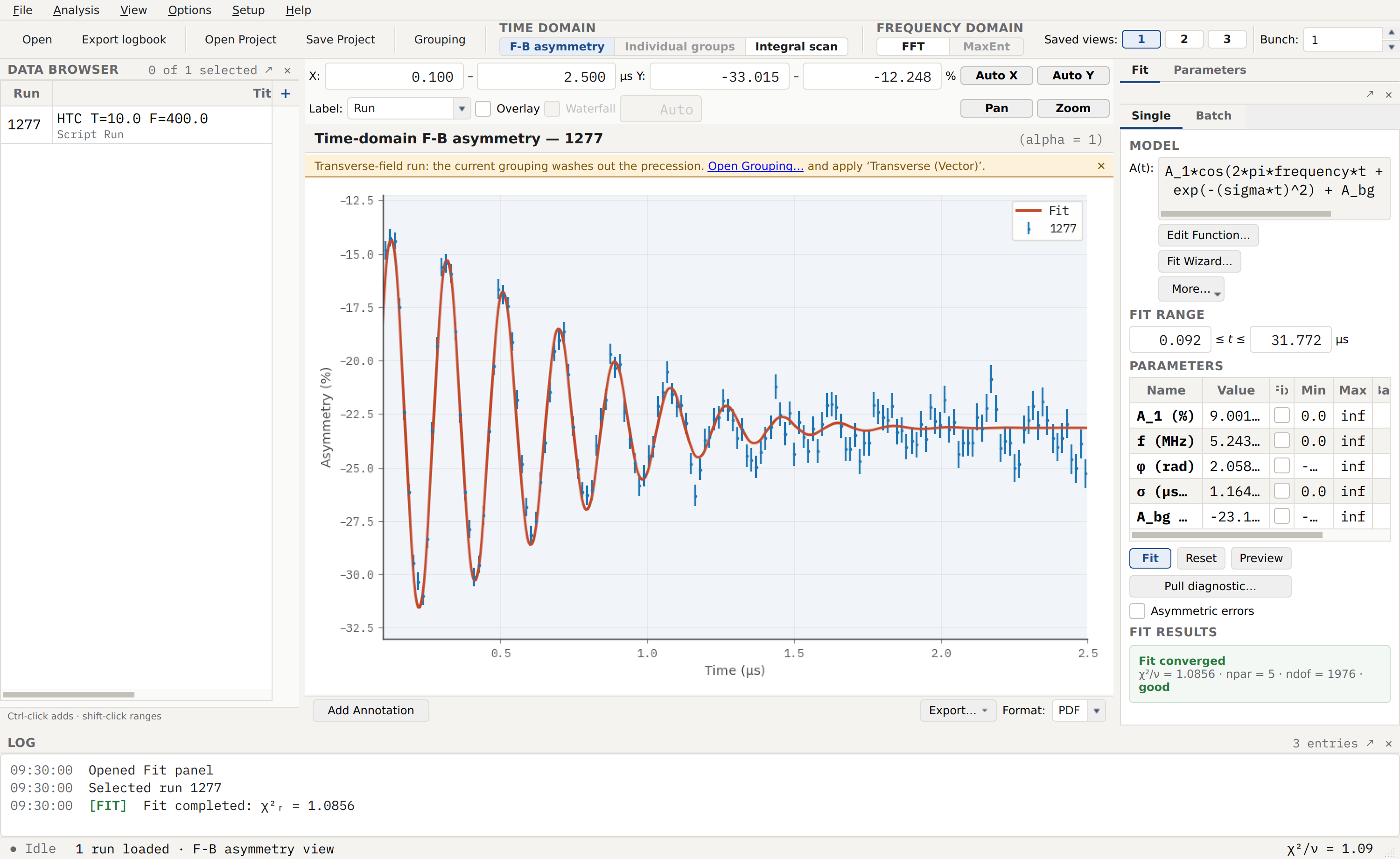
The Fit dock (Single tab) after fitting the base-temperature
400 G run (1277, 10 K). The composite model
Oscillatory * Gaussian + Constant —
A_1*cos(2*pi*frequency*t)*exp(-(sigma*t)^2) + A_bg in the MODEL
box — carries the vortex signal: the oscillation at the 400 G Larmor
frequency (f = 5.24 MHz, shifted below the applied field by the
diamagnetic response) under a Gaussian envelope that collapses the
precession within ~2 μs. The PARAMETERS table reports
σ = 1.164 μs⁻¹, and FIT RESULTS shows “Fit converged” with
\(\chi^2_\nu = 1.09\).
For each temperature the per-run recipe is the same. Open the Fit dock,
build the composite Oscillatory * Gaussian + Constant in the function
builder (see Composite models), and record the Gaussian
envelope’s \(\sigma\) — the second moment of \(p(B)\) — with its
uncertainty. The Oscillatory component carries the average field’s
Larmor frequency; the additive Constant absorbs the non-precessing
baseline. The fitted σ = 1.164 μs⁻¹ reproduces the WiMDA reference
value of 1.1467(75) μs⁻¹ for this run to within about 1.5 %, and the
agreement holds to a few per cent across the superconducting range of the
scan. (Asymmetry delivers the loader’s forward/backward asymmetry rather
than WiMDA’s full eight-group grouping, which is the source of the small
residual offset.)
Step 2 — Inspect the vortex line shape
The guide asks the analyst to compare the time-domain fit with the frequency-domain line shape, first by FFT and then by maximum entropy. Both views make the vortex broadening directly visible.
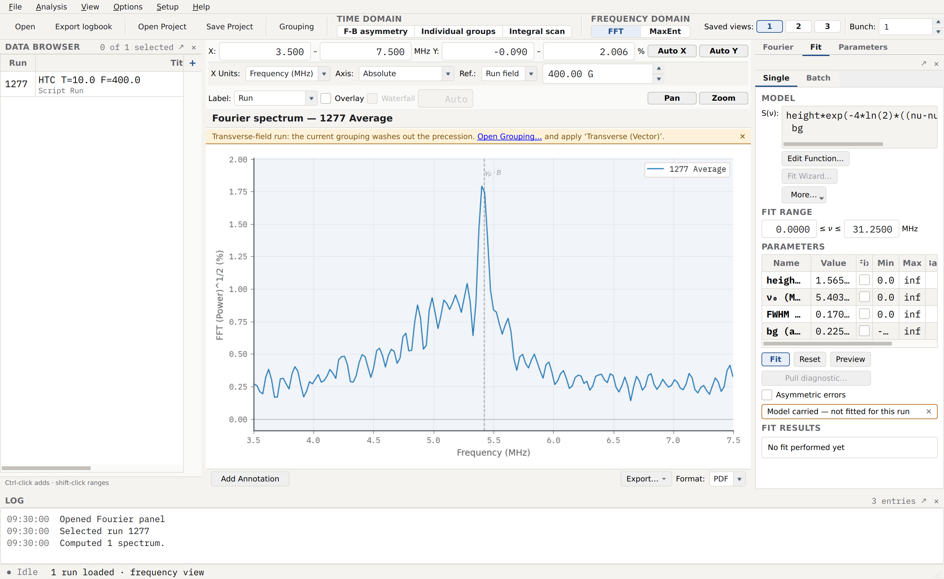
The Frequency domain (FFT under FREQUENCY DOMAIN) of the
10 K run. With X Units: Frequency (MHz) and Reference:
400.00 G, the broad, asymmetric vortex line sits on the 400 G Larmor
frequency near 5.4 MHz — the frequency-domain image of the mixed-state
\(p(B)\). Its width is the same second moment the time-domain
Gaussian \(\sigma\) measures; above \(T_c\) this line collapses
to a narrow nuclear-dipolar Gaussian.
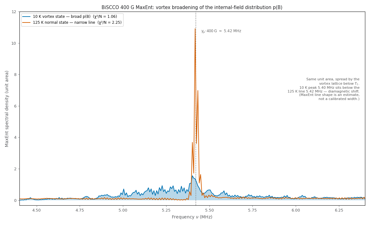
The maximum-entropy (MaxEnt) reconstruction, the guide’s FFT-versus-MaxEnt comparison. The 10 K vortex distribution (filled, \(\chi^2/N = 1.04\)) spreads the same unit spectral area that the 125 K normal-state line concentrates into a single narrow peak — the vortex lattice broadening \(p(B)\). The 10 K peak (5.40 MHz) sits just below the normal-state line (5.42 MHz): the diamagnetic shift of the mixed state. On this real forward/backward asymmetry the estimator converges out of the box, seeding the four MUSR quadrant-group phases from the data — the Seed phases from data option, on by default.
Note
A maximum-entropy line shape is a regularised estimate of \(p(B)\), not a calibrated linewidth. Treat the MaxEnt and FFT views as qualitative pictures of the broadening; the quantitative \(\sigma\) comes from the time-domain Gaussian fit of Step 1.
Step 3 — Trend σ(T) through T_c
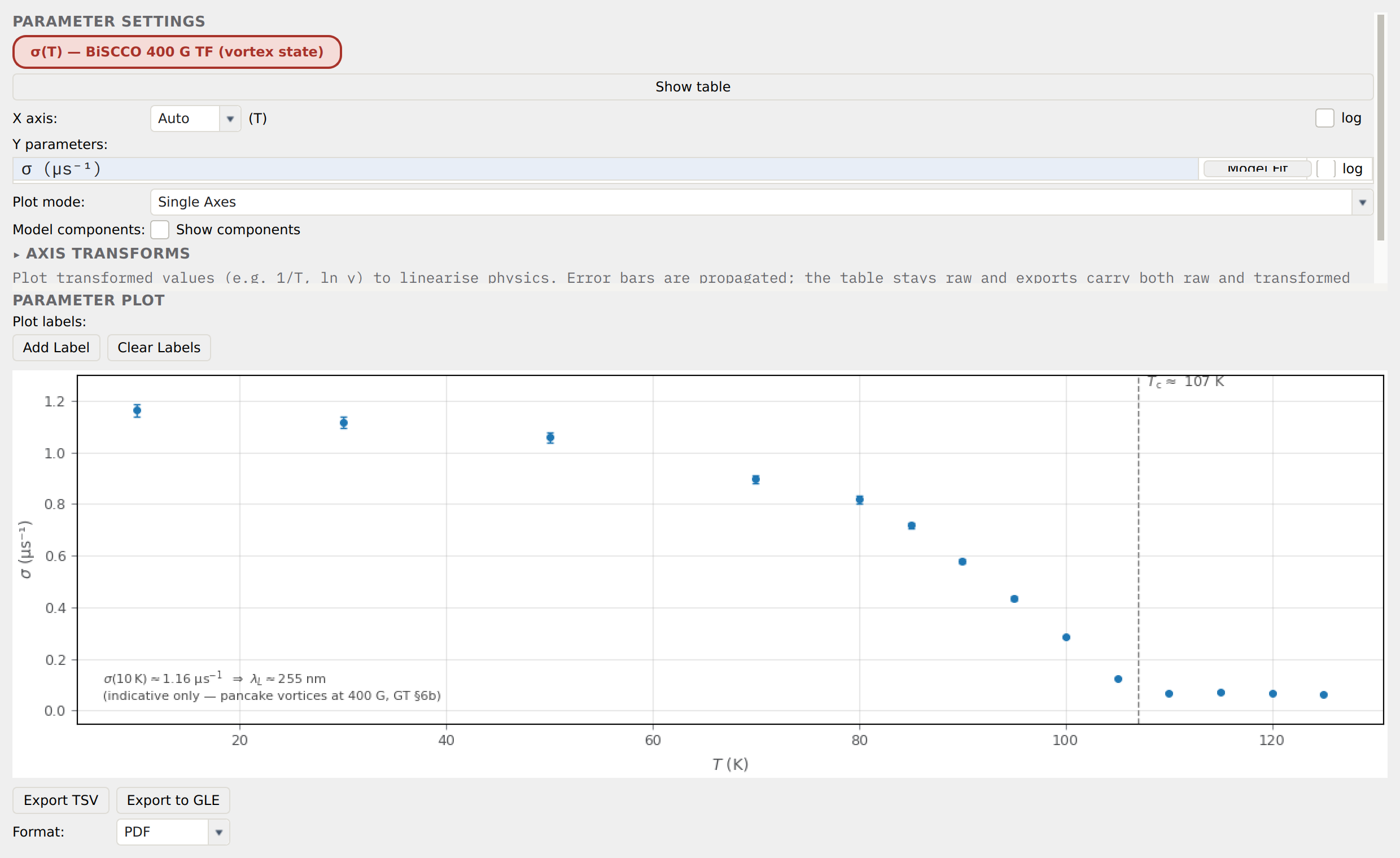
The Fit Parameters trend panel with the per-run 400 G
\(\sigma(T)\) series loaded and σ (µs⁻¹) on the y-axis. The
points reproduce the 14-row WiMDA reference trend: \(\sigma\) falls
from ≈ 1.16 μs⁻¹ at 10 K to a small residual ≈ 0.06 μs⁻¹ above
\(T_c \approx 107\;\mathrm{K}\). The base-temperature value maps to
\(\lambda_L = \sqrt{75780/\sigma} \approx 255\;\mathrm{nm}\) — noted
on the plot as indicative only (see below).
Loading each run’s fit result into the trend panel and selecting
σ (µs⁻¹) from Y parameters plots the depolarisation rate against
temperature. The curve has the canonical mixed-state form: a low-\(T\)
plateau where the superfluid density is fully developed, a monotonic fall
on warming as \(\rho_s\) melts, and a collapse to the nuclear-dipolar
background as superconductivity is lost near 107 K. The lowest-\(T\)
value, \(\sigma(10\;\mathrm{K}) \approx 1.16\;\mu\mathrm{s}^{-1}\),
gives \(\lambda_L \approx 255\;\mathrm{nm}\) through the guide relation,
consistent with the reference σ (257 nm) and the literature order of
magnitude for optimally-doped Bi-2212 (\(\lambda_{ab} \approx
260\;\mathrm{nm}\)).
Warning
A single :math:`lambda_L` is only indicative for Bi-2212 at these fields. Bi-2212 is extremely anisotropic, and above a crossover field \(B^* \approx 500\;\mathrm{G}\) its flux lines break into weakly correlated pancake vortices. All three teaching fields (150, 200 and 400 G) sit below \(B^*\), so the extended-flux-line interpretation of \(\sigma\) as \(\lambda_{ab}\) is not physically robust here (see Bernhard et al., Phys. Rev. B 52, 10488 (1995), which states that meaningful \(\lambda_{ab}\) values “cannot be extracted from \(\sigma\)” in the usual way for this material). Quote \(\lambda_L \approx 255\;\mathrm{nm}\) as an order-of-magnitude guide from \(\lambda_L = \sqrt{75780/\sigma}\), and grade the \(\sigma(T)\) curve itself rather than a single derived \(\lambda_L\).
Step 4 — Compare the two fields
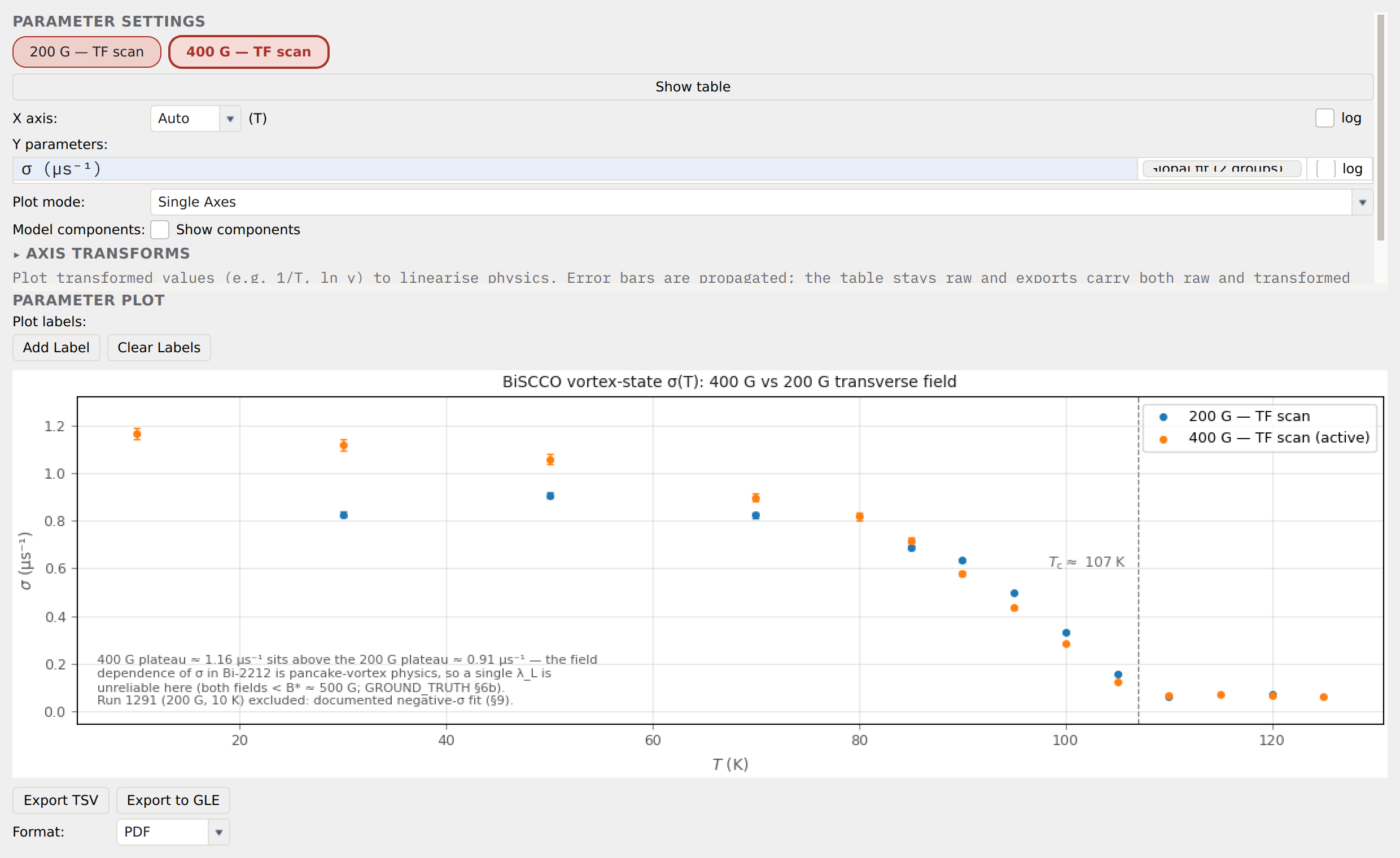
The trend panel overlaying the 400 G and 200 G \(\sigma(T)\) scans
as two coloured series (armed through select_series, the equivalent
of Shift-clicking the second series pill). Both are genuine per-run TF
Gaussian fits. The 200 G plateau (≈ 0.9 μs⁻¹) sits below the 400 G
plateau (≈ 1.15 μs⁻¹): the field dependence of \(\sigma\) in Bi-2212
is the pancake-vortex physics of the warning above, not fit scatter. The
10 K, 200 G run (1291) is excluded — its reference fit is a documented
negative-\(\sigma\) pathology.
The guide’s field-comparison task is exactly this overlay. For a conventional, weakly-anisotropic superconductor deep in the mixed state, \(\sigma\) is field-independent between \(H_{c1}\) and \(H_{c2}\), and the two scans would coincide. That they do not is the signature of dimensional crossover: below \(B^*\) the pancake vortices in adjacent CuO₂ planes decouple, the lattice order softens, and the measured second moment shrinks. The overlay is a plot-only comparison; Export TSV writes both series, while GLE export and any trend Model Fit apply to the active series alone.
Fitting a gap model
Where the material and the field permit a clean single-\(\lambda\) interpretation — which Bi-2212 at 150–400 G does not — the next step is to fit the superfluid density \(\sigma(T)\) (background-subtracted) to a gap model and read off the pairing symmetry. Asymmetry’s parametric-model registry ships the standard family, each documented in the component-info dialog:
SC_SWave— a single isotropic, fully-gapped BCS order parameter; \(\sigma(T)\) saturates exponentially at low \(T\).SC_DWave— a nodal d-wave gap; the line nodes give \(\sigma(T)\) a linear low-\(T\) slope rather than activated saturation.SC_TwoGap_SS— two nodeless gaps for multiband superconductors (the MgB₂-type case), with a weight partitioning the superfluid density between the two channels.SC_TwoGap_SD— a mixed s + d interpretation for cases where neither pure form fits the full temperature range.
The _Q variants (SC_SWave_Q, SC_DWave_Q) combine the
superconducting and normal linewidth contributions in quadrature rather
than linearly, appropriate when the two sources are independent. Fit these
in the trend panel by selecting σ (µs⁻¹) and clicking Model Fit, or
export the trend (Export TSV) and fit outside the GUI with
scipy.optimize.curve_fit. In every case, include a few points above
\(T_c\) so the high-\(T\) tail anchors both \(T_c\) and the
nuclear-dipolar background \(\sigma_{bg}\), and subtract
\(\sigma_{bg}\) in quadrature before converting \(\sigma \to
\lambda\).
Cross-reference — LiFeAs, the field width B_rms(T)
The LiFeAs corpus example runs the same vortex-lattice workflow on the “111” iron-arsenide superconductor, but reports the linewidth as a field width \(B_\mathrm{rms} = \sigma_\mathrm{VL}/\gamma_\mu\) (mT) rather than a rate, following Pratt et al., Phys. Rev. B 79, 052508 (2009). The superconducting broadening adds in quadrature to a temperature-independent nuclear width, \(\sigma^2 = \sigma_\mathrm{VL}^2 + \sigma_n^2\), and the powder London limit gives \(B_\mathrm{rms} = \sqrt{0.00371}\,\Phi_0/(3^{1/4}\lambda_{ab})^2\).
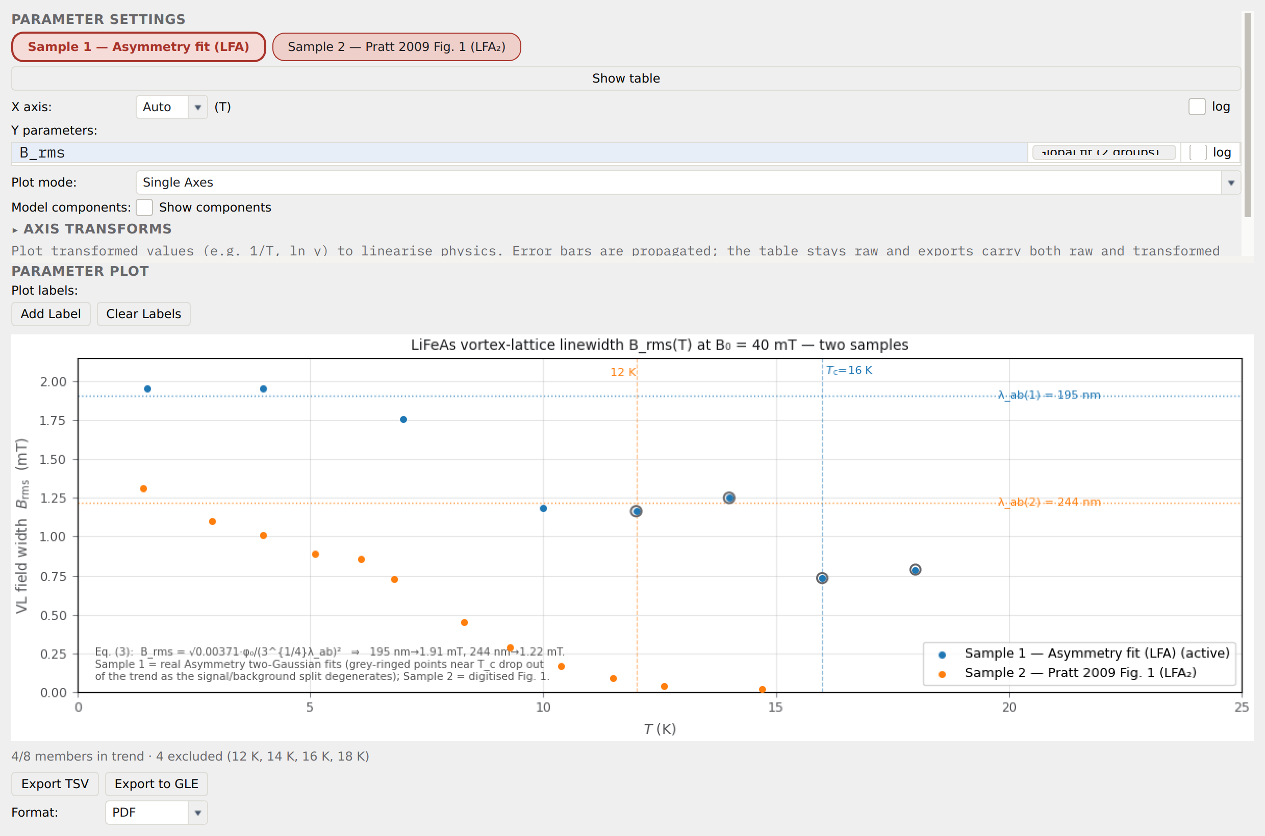
\(B_\mathrm{rms}(T)\) at \(B_0 = 40\;\mathrm{mT}\) for two LiFeAs samples overlaid in the trend panel: Sample 1 (real Asymmetry two-Gaussian fits, \(T_c = 16\;\mathrm{K}\), plateau ≈ 1.9 mT) against Sample 2 (digitised from the paper’s Fig. 1, \(T_c \approx 12\;\mathrm{K}\), ≈ 1.2 mT). The dotted lines mark the London-limit plateaux for the printed \(\lambda_{ab} = 195(2)\;\mathrm{nm}\) and \(244(2)\;\mathrm{nm}\). Points near \(T_c\), where the signal/background split degenerates, are ringed grey and drop out of the trend.
Cross-reference — Re₆Zr, superfluid density and a TRSB step
The TRSB corpus example (Re₆Zr, a noncentrosymmetric superconductor; Singh, Hillier et al., Phys. Rev. Lett. 112, 107002 (2014)) carries two observables. The transverse-field superfluid density behaves exactly as above, while a separate zero-field measurement reveals broken time-reversal symmetry.
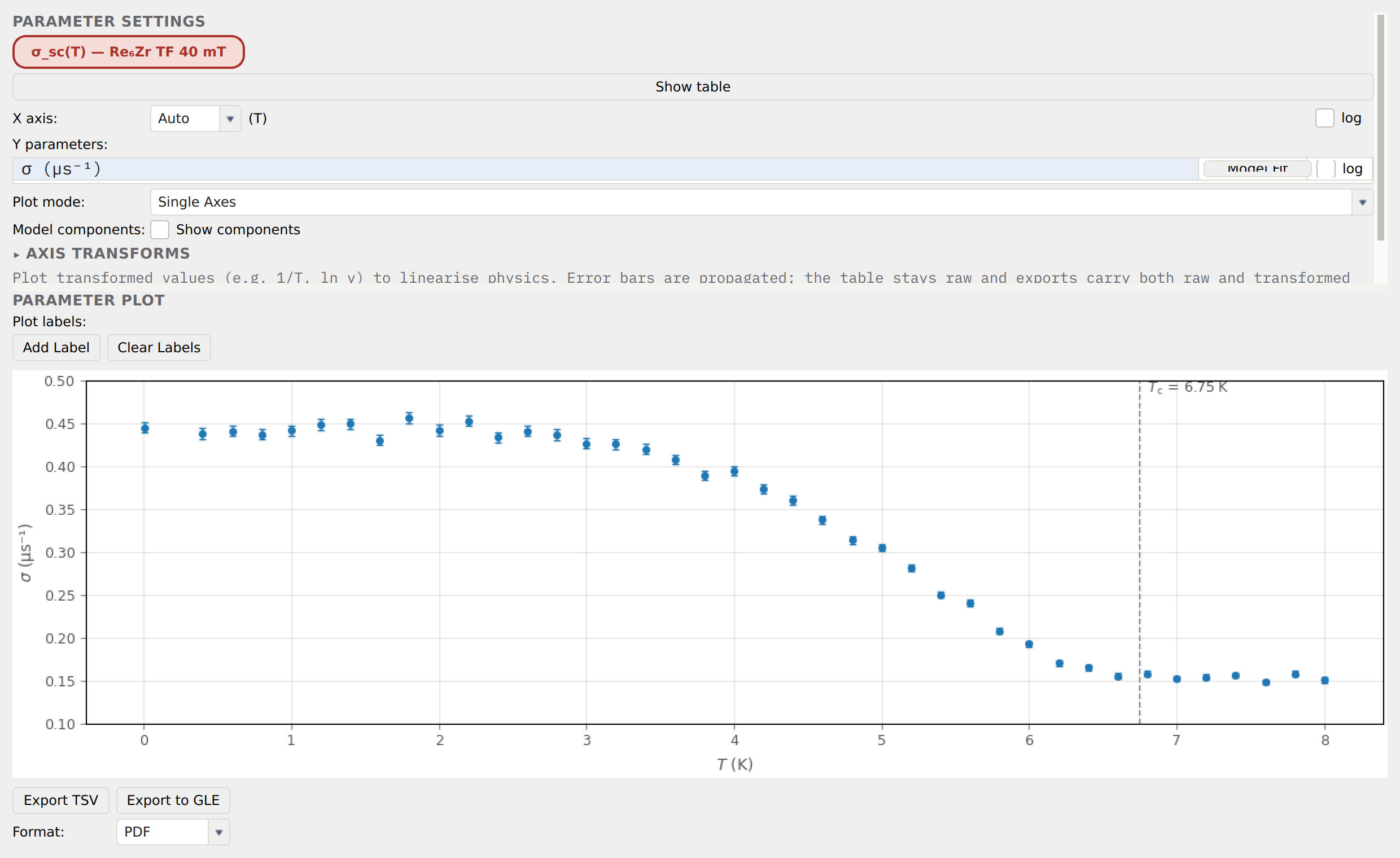
The TF depolarisation rate \(\sigma_{sc}(T)\) at 40 mT, falling from ≈ 0.45 μs⁻¹ at base temperature toward a ≈ 0.17 μs⁻¹ normal-state plateau through \(T_c = 6.75\;\mathrm{K}\). The low-\(T\) plateau and the melt between ~3 and ~7 K are the s-wave superfluid-density signature, reproducing the WiMDA reference trend.
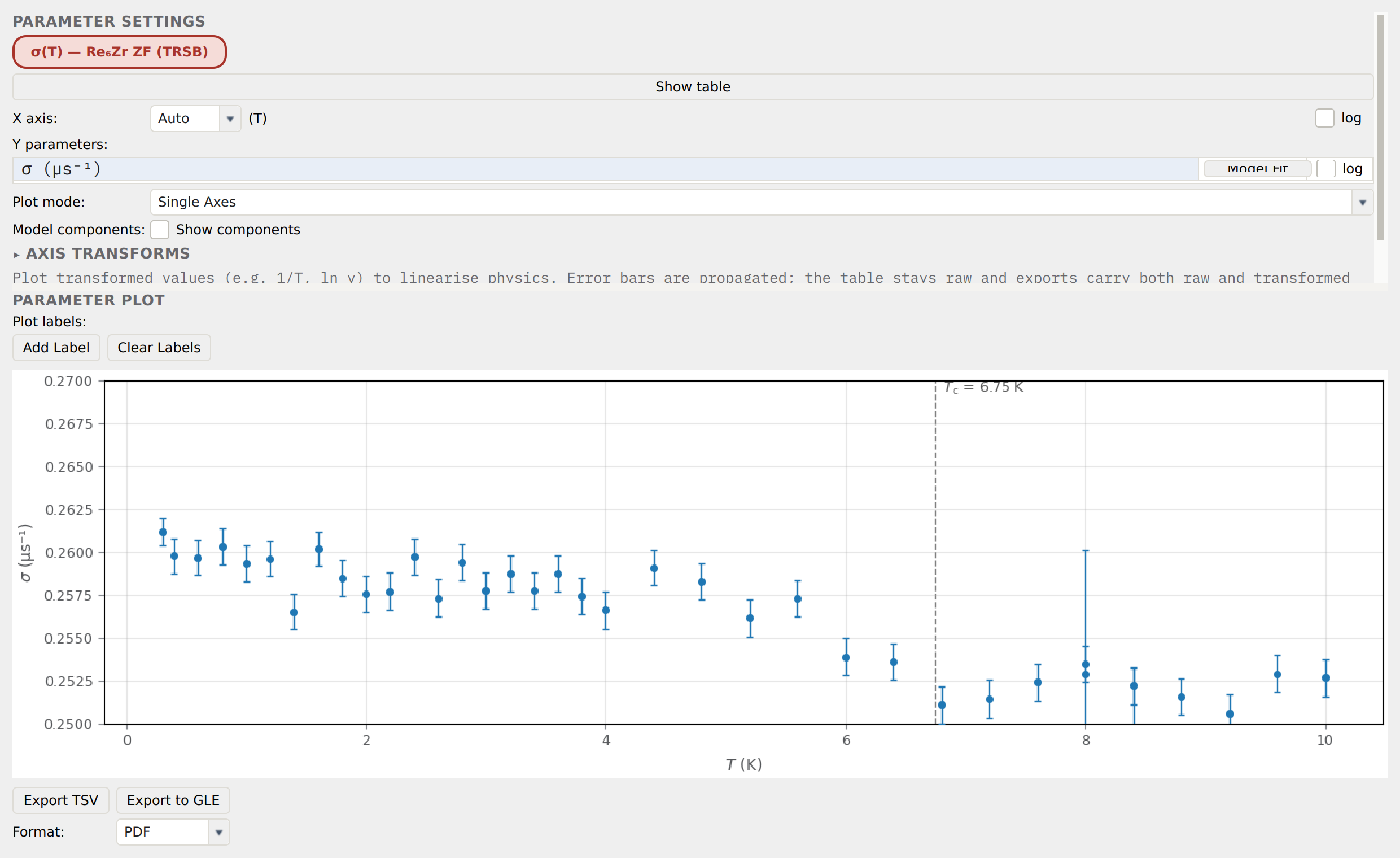
The zero-field Gaussian Kubo–Toyabe rate \(\sigma(T)\), framed on a tight 0.250–0.270 μs⁻¹ axis to resolve the small spontaneous rise below \(T_c = 6.75\;\mathrm{K}\) (\(\Delta\sigma \approx 0.006\text{–}0.01\;\mu\mathrm{s}^{-1}\)). The onset of static spontaneous fields at \(T_c\) — decoupled by a 10 mT longitudinal field — is the time-reversal-symmetry-breaking signature. Unlike the TF superfluid density, this small zero-field step is the headline physics of that example, and Asymmetry renders it legibly only because the axis is framed to the signal.
Interpretation
What the shape of \(\sigma(T)\) (equivalently \(\rho_s(T)\)) tells you about the material:
Exponential low-:math:`T` saturation. A single isotropic s-wave gap (
SC_SWave); the \(\Delta/k_B T_c\) value distinguishes weak-coupling (BCS, 1.764) from strong-coupling (Re₆Zr reaches 2.1).Linear-in-:math:`T` low-:math:`T` decrease. Line nodes in the gap (
SC_DWave); the hallmark of a d-wave order parameter, as in the cuprates.A shoulder or kink near :math:`T/T_c approx 0.3text{–}0.5`. Multiband superconductivity with two gaps (
SC_TwoGap_SS); the smaller gap freezes out at its own scale.A field-dependent plateau. As in Bi-2212 here: not a pairing-symmetry statement at all, but dimensional-crossover physics that invalidates a single-\(\lambda\) reading.
Assumptions and limitations
The London limit. \(\sigma \to \lambda\) is exact only for \(\lambda \gg \xi\). Where \(\xi\) approaches \(\lambda\) the Brandt expression acquires corrections (see Sonier et al., Rev. Mod. Phys. 72, 769 (2000), Appendix B).
The nuclear-dipolar background. Even above \(T_c\) the muon sees a non-zero \(\sigma\) from nuclear dipoles (≈ 0.055 μs⁻¹ here). Fit it and subtract it in quadrature before converting \(\sigma \to \lambda\).
Anisotropy and the vortex regime. Below \(H_{c1}\) the field does not enter as a lattice; above \(H_{c2}\) superconductivity is suppressed; and in extremely anisotropic layered materials a pancake- vortex crossover (Bi-2212 above) breaks the single-\(\lambda\) picture even well inside the mixed state.
Convention on the absolute :math:`lambda`. The guide’s coefficient (75780) and the Brandt/Bernhard form differ by ~7 %, so the absolute \(\lambda_L\) is convention-dependent at the ~10 % level; the shape of \(\lambda_L(T)\) is not.
Data range. Without points above \(T_c\) the fit cannot separate \(T_c\) from \(\sigma_{bg}\); without points below \(T/T_c \approx 0.3\) a small gap in a two-gap model is poorly constrained.
References
References
E. H. Brandt, Phys. Rev. B 37, 2349 (1988) — the vortex-lattice field distribution and its second moment.
J. E. Sonier, J. H. Brewer, and R. F. Kiefl, Rev. Mod. Phys. 72, 769 (2000) — the canonical review of TF μSR in superconductors.
C. Bernhard, Ch. Niedermayer, U. Binninger, A. Hofer, Ch. Wenger, J. L. Tallon, G. V. M. Williams, E. J. Ansaldo, J. I. Budnick, C. E. Stronach, D. R. Noakes, and M. A. Blankson-Mills, Phys. Rev. B 52, 10488 (1995) — the σ ↔ λ relation and the pancake-vortex caveat for Bi-2212.
F. L. Pratt, P. J. Baker, S. J. Blundell, T. Lancaster, H. J. Lewtas, P. Adamson, M. J. Pitcher, D. R. Parker, and S. J. Clarke, Phys. Rev. B 79, 052508 (2009) — LiFeAs \(B_\mathrm{rms}(T)\) and \(\lambda_{ab}\).
R. P. Singh, A. D. Hillier, B. Mazidian, J. Quintanilla, J. F. Annett, D. McK. Paul, G. Balakrishnan, and M. R. Lees, Phys. Rev. Lett. 112, 107002 (2014) — Re₆Zr TRSB and superfluid density.
S. J. Blundell, R. De Renzi, T. Lancaster, and F. L. Pratt, Muon Spectroscopy: An Introduction (Oxford University Press, Oxford, 2022), Ch. 9 (superconductors), especially Ch. 9.5 (penetration depth and gap structure).
A. Amato and E. Morenzoni, Introduction to Muon Spin Spectroscopy: Applications to Solid State and Material Sciences, Lecture Notes in Physics Vol. 961 (Springer, Cham, 2024), Ch. 6 — the vortex-state field distribution, multiband superconductivity, and unconventional pairing.
Cross-references
Loading Data — loading the ISIS
.nxsand PSI.bincorpus runs.Detector Grouping and Layout — the transverse (Up/Down) grouping choice for spin-rotated runs.
Composite models — building the
Oscillatory * Gaussian + Constanttime-domain composite.Fourier analysis — inspecting the \(p(B)\) line shape by FFT and maximum entropy.
Parameter trending — the σ → λ → gap-model pipeline and multi-series overlays.
Superconducting penetration depth models — the parametric
SC_*gap-model reference page.