EMU detector grouping and α calibration

This is the recommended first walkthrough for new users. It covers the everyday setup every time-domain analysis depends on: loading a run, defining the forward/backward detector grouping, calibrating \(\alpha\) from a transverse-field (TF) run, turning on dead-time correction, and reading the timing origin \(t_0\) and good-data window — all built into one named grouping profile for the instrument, edited from the Grouping window. It closes with the fit-table trend that turns a run series into a single answer.

It is the Asymmetry-worded counterpart to the WiMDA muon-school “Basics” exercise, worked on the same teaching data. Where WiMDA asks you to type a detector list into a text box, Asymmetry gives you a visual Detector Layout Editor with instrument presets, and collects every calibration field — \(t_0\), good-data window, dead-time, grouping, and \(\alpha\) — under one profile, with each correction calibrated in its own dedicated dialog.

The runs

The walkthrough draws on the corpus Basics set (Basics/data/, the ISIS muon-school data-handling primer, stored as HDF4 NeXus and read natively). Each calibration concept is shown on the run where it reads most clearly:

Run	Instrument / sample	Role
MUSR00044989	MuSR — Ag on candlestick	Detector grouping — 64 detectors summed into two groups (Step 2).
EMU00018854	EMU — silver, 100 G TF	\(\alpha\) calibration from a clean transverse-field run (Step 3).
emu00034998	EMU — silver, high count rate	Dead-time correction, Off versus loaded (Step 5).
EMU00018850	EMU — silver, TF	\(t_0\) and the good-data window (Step 6).
EMU00044989–44997	EMU — Ag mask on Fe₂O₃, 100 G TF	Steering-current trend across a run series (Step 7).

Silver is the standard calibrant: it has a near-zero nuclear moment, so a small transverse field produces a clean, slowly-relaxing precession whose forward/backward amplitudes reveal any detector imbalance, and its well-characterised response makes it the reference sample for both \(\alpha\) and per-detector dead-time.

Step 1 — Load a run

Open a run from File → Open (or drag it onto the window). The Data Browser lists one row per run; the central plot shows the currently-selected run’s asymmetry. Loading several files at once is fine — any run of this instrument assigned to the profile follows what you build below automatically, with no separate step to push it out to the rest of the series.

Step 2 — Open the Grouping window

Click Grouping on the toolbar (or Analysis → Grouping…) and create a profile for the instrument (or pick an existing one). The window is the whole calibration surface for that profile:

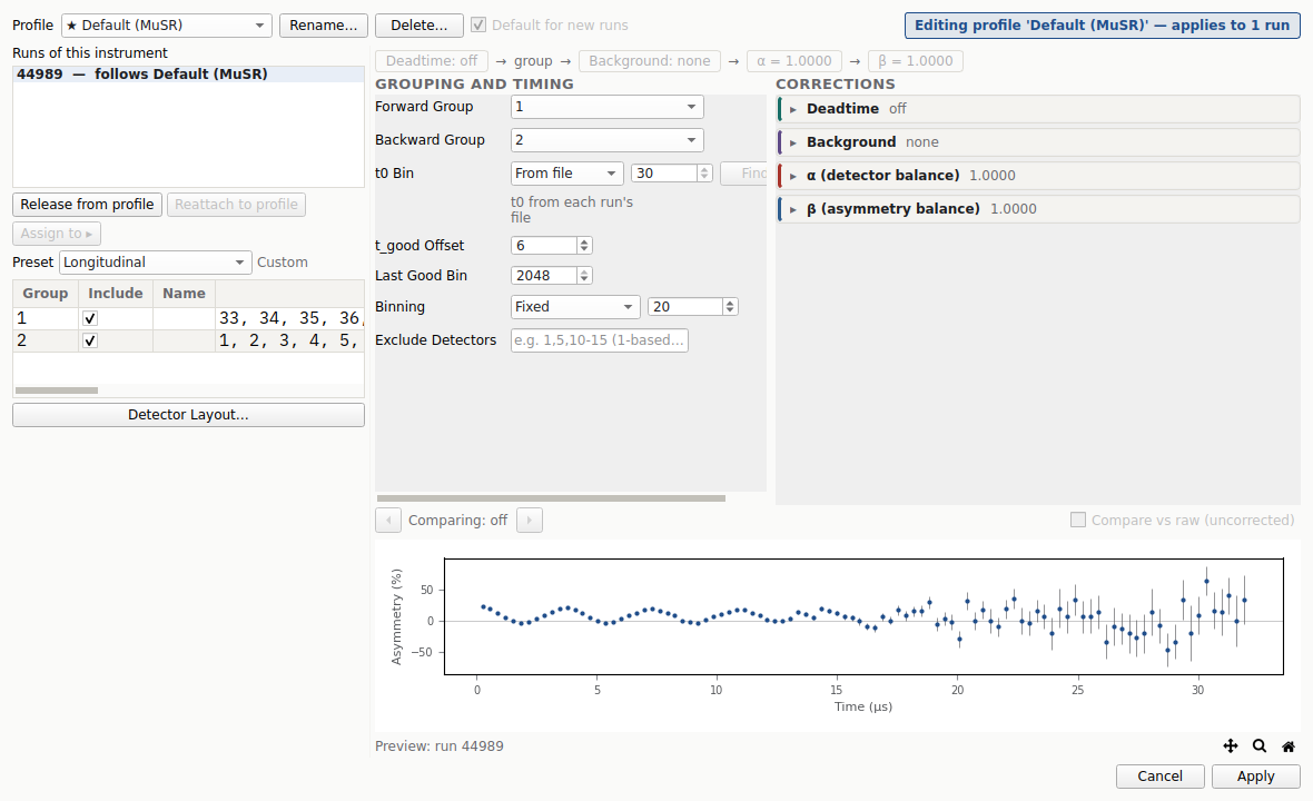
The Grouping window on the muon-school grouping run MUSR00044989 (Ag on candlestick), where the MuSR spectrometer’s 64 detectors are the clearest demonstration of grouping. The group table on the left sums the detectors into two groups of 32 — one holding detectors 1–32, the other 33–64 — and the Forward Group / Backward Group selectors pair them into the \(F\) and \(B\) sums (here 33–64 forward, 1–32 backward). Alpha still reads 1.000000 · manual because the run has not yet been calibrated; t0 Bin shows From file = 30 with t_good Offset = 6 and Last Good Bin = 2048, all seeded from the file header; Deadtime is off. The live asymmetry along the bottom redraws as you change any of these. (The amber banner is an advisory heuristic that misreads this zero-field run as transverse; it is only a suggestion — the grouping shown is correct.)

Field	What it sets
Profile selector	Which named profile you are editing, with Rename… to relabel it.
Scope panel (“Runs of this instrument”)	Every run of this instrument, tagged follows <profile> or override. This is the selector: the run you pick here is the one the form previews and edits, and its per-run facts (\(t_0\), good-bin window, file dead-time) seed the status rows. Release from profile / Reattach to profile move a run between inheriting the profile and carrying its own override.
Editing-target strip	A strip above the form that names what your edits currently apply to — “Editing profile ‘<name>’ — applies to N runs” while an inheriting run is selected, or the override wording while an overridden run is selected.
Forward Group / Backward Group	Which detector groups form the \(F\) and \(B\) sums of the asymmetry.
Alpha / Calibrate…	The current \(\alpha\) and its provenance, with a Calibrate… button that opens the alpha calibration dialog (see Step 3).
t0 Bin	The time-zero bin (the muon-implantation prompt), with a mode selector — From file (the default), Manual, or Auto-detect — and a Find t0 button for the automatic search.
t_good Offset	First good bin, measured as an offset after \(t_0\).
Last Good Bin	End of the good-data window.
Binning	Time-bin rebinning; the Fixed mode merges a fixed number of raw bins (the bunching factor, also available on the toolbar).
Exclude Detectors	A list of detector ids to drop from every group (masked or dead tubes).
Deadtime / Configure…	Opens the deadtime dialog: mode (Off / From file / Manual / Estimate from run), per-detector table, Cal fit (see Step 5).
Background / Configure…	Opens the background dialog for a constant-background subtraction.
Live preview	The forward/backward asymmetry the current draft would produce, updating as you edit.
Detector Layout…	Opens the visual editor and instrument presets (see Step 4).
Apply	Write the draft back to the profile — and any edited overrides to their own runs, in one pass. The Log echoes how many inheriting runs it reached.

Step 3 — Calibrate α from the TF run

In the α (detector balance) card of the Corrections column, pick the silver TF calibration run (EMU00018854, silver in a 100 G transverse field) from the Calibration run dropdown. Because this run’s field geometry is transverse and its magnitude sits in the weak-TF window, it is highlighted and pre-selected there. Choose a Method and press Estimate α.

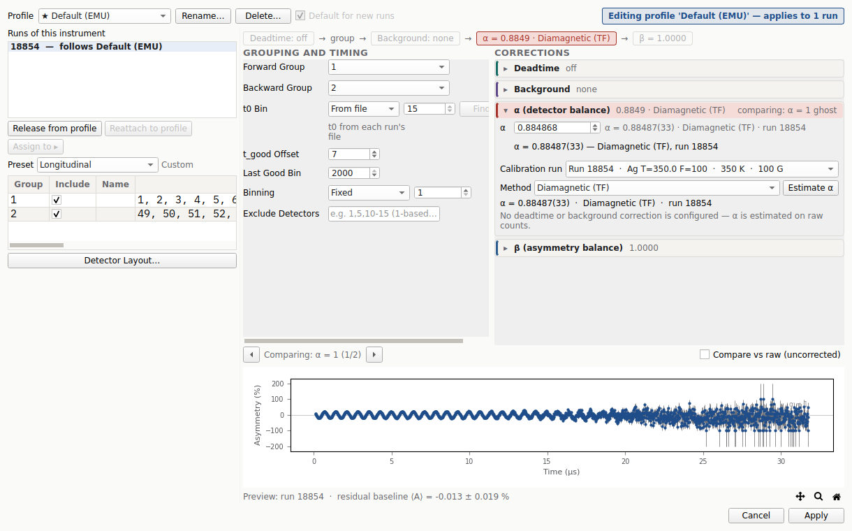
The inline alpha calibration on the silver TF run EMU00018854. With the Diamagnetic (TF) method and the good-bin window 21–1999, pressing Estimate α returns \(\alpha = 0.88487(33)\), reported in the α card as α = 0.88487(33) · Diamagnetic (TF) · run 18854. The shared preview overlays the uncorrected asymmetry (grey, \(\alpha = 1\)) on the calibrated one (blue): the fitted \(\alpha\) pulls the precession down onto a symmetric oscillation about zero, removing the forward/backward imbalance.

Choose the Diamagnetic (TF) method. On a silver TF run the precession is a clean, non-relaxing oscillation, and the correct \(\alpha\) is the one that makes the forward/backward asymmetry oscillate symmetrically about zero — an imbalanced \(\alpha\) leaves the precession riding on a non-zero offset. Asymmetry finds it by minimising the weighted asymmetry power over the good-data window,

\[\alpha = \arg\min_\alpha \sum_i \left(\frac{A_i}{\sigma_i}\right)^2, \qquad A_i = \frac{F_i - \alpha B_i}{F_i + \alpha B_i},\]

with \(\sigma_i\) the Poisson-propagated per-bin asymmetry error — WiMDA’s diamagnetic estimate. The Count ratio ΣF/ΣB method instead computes the simple integral balance \(\alpha = \sum_i F_i / \sum_i B_i\) (Mantid’s AlphaCalc), with no oscillation model; on a clean silver run the two agree closely. The General (LF/ZF) method balances lifetime-corrected counts and accommodates a genuinely relaxing signal, but needs visible relaxation. On this silver TF run the diamagnetic estimate gives \(\alpha = 0.88487(33)\), and the shared before/after preview shows the balancing effect directly. The estimate applies immediately: the α card reads α = 0.88487(33) · Diamagnetic (TF) · run 18854.

The same calculation is available from the Python API. The diamagnetic fit lives in estimate_alpha_detailed(); the simpler integral ratio (equivalent to the Count ratio ΣF/ΣB method) is estimate_alpha():

from asymmetry.core.io import load
from asymmetry.core.transform import apply_grouping, estimate_alpha_detailed

tf = load("Basics/data/EMU00018854.nxs")
g = tf.run.grouping
groups = g["groups"]                             # {group_id: [1-based detector ids]}
fwd = [int(d) - 1 for d in groups[g["forward_group"]]]
bwd = [int(d) - 1 for d in groups[g["backward_group"]]]
forward = apply_grouping(tf.run.histograms, fwd)
backward = apply_grouping(tf.run.histograms, bwd)
est = estimate_alpha_detailed(
    forward, backward,
    method="diamagnetic",
    first_good_bin=g.get("first_good_bin"),
    last_good_bin=g.get("last_good_bin"),
)
print(round(est.alpha, 3))                        # 0.885

Press Apply to write the calibrated \(\alpha\) back to the profile. Any run of the same instrument assigned to the profile follows it — grouping and \(\alpha\) included — the moment it is loaded (see Reusing the calibration below), so nothing further needs to be selected or applied on it by hand. Note, though, that \(\alpha\) is a sample calibration: carry it only to runs of the same sample and detector arrangement.

Step 4 — The visual Detector Layout Editor

Click Detector Layout… to open the visual editor — Asymmetry’s replacement for WiMDA’s “edit detector list” text box. It draws the instrument’s physical forward and backward detector arrays as concentric rings of segments:

The Detector Layout editor on EMU’s Longitudinal preset — the two-group forward/backward split this exercise uses. The preset dropdown seeds the arrangement; clicking a segment toggles its membership in the active group. (Shown here on EMU for its longitudinal geometry; the grouping window above is the same editor reached from any loaded instrument.)

• Click a segment to toggle its membership in the active group. Colours and names distinguish up to eight groups, each showing a live member count, and a detector may belong to more than one group — drawn as its own thin slice per membership.

• Hover a detector for its id, physical label, group memberships, and exclusion state.

• The preset grouping dropdown offers instrument-aware layouts. For EMU these are Longitudinal (the standard two-group F/B split used here) and Vector Polarization (the multi-axis layout used for Vector-polarisation mode).

For this silver exercise the Longitudinal preset is the correct starting point; the editor is most useful when a detector is masked or when you build a custom geometry. See Detector Grouping and Layout for the full reference.

Step 5 — Dead-time correction

After a detector records a positron there is a short interval before it can register the next; at the high instantaneous rates of a pulsed source a positron arriving inside that interval is lost, and the count must be statistically recovered. The per-detector dead-times are measured once from a silver sample and stored in the data file (Kilcoyne, RAL-94-080).

Click Configure… beside the Deadtime row and choose a mode:

• From file — use the per-detector dead-time values stored in the data file (the usual choice, and WiMDA’s “Auto Load”).

• Manual — type per-detector values (in ns), or paste a calibration.

• Estimate from run — fit the dead-time from the early-time count rate; the Cal button fits one value per detector from the preview run.

The dialog also reports “Max correction at t=0”, the largest correction any detector receives, so an unreasonable value is visible immediately.

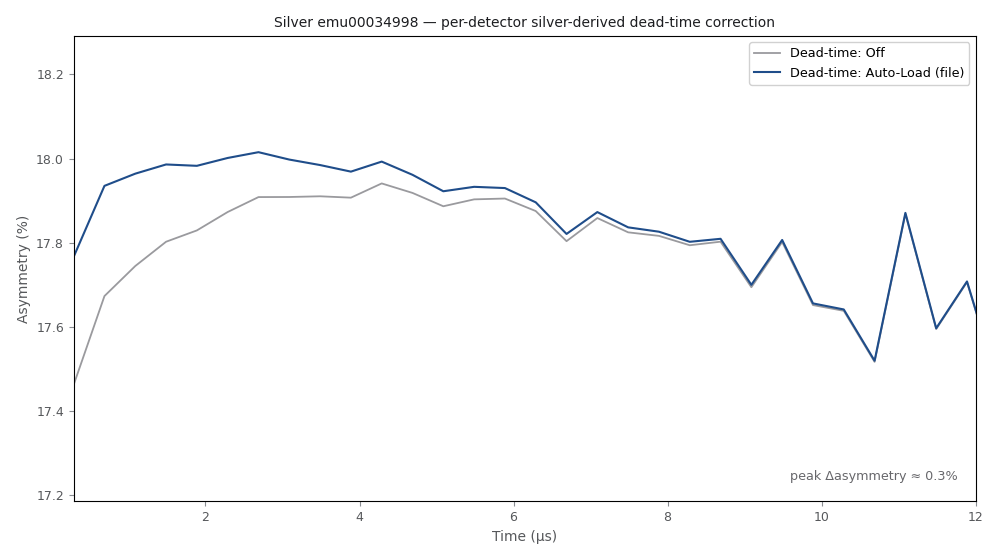
The muon-school “show the effect” plot on the high-rate silver run emu00034998: the forward/backward asymmetry with dead-time Off (grey, near 17.8 %) and with the per-detector silver-derived correction loaded From file (blue, near 23 %). On this deliberately high-rate run the correction is a visible ≈ 5.2 % early-time shift, not a sub-percent tweak — which is exactly why silver at a high rate is the run the exercise uses to make dead-time visible. On a well-behaved low-rate histogram the same correction is far smaller.

Step 6 — Timing: t0 and the good-data window

At a pulsed source the timing origin \(t_0\) is when the middle of the muon pulse reaches the sample. The good data do not begin until the whole pulse has arrived — that time is \(t_\text{good}\), and the difference \(t_\text{good} - t_0\) is the good-data offset. Both are normally read straight from the file (the instrument scientist sets them), which is what t0 Bin → From file does; you rarely edit them, but it helps to see what they mark.

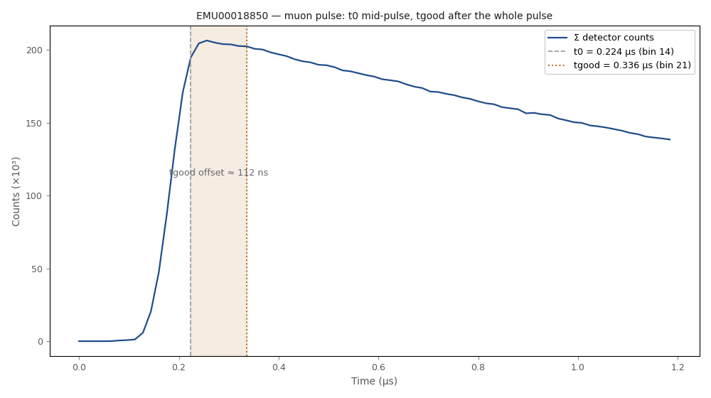
The summed detector counts of the silver run EMU00018850 through the muon pulse. The prompt rises over roughly 0.1 µs; the stored \(t_0 = 0.224\ \mu\text{s}\) (bin 14) sits at the mid-pulse and the stored \(t_\text{good} = 0.336\ \mu\text{s}\) (bin 21) sits after the whole pulse has passed, leaving a good-data offset of ≈ 112 ns — the finite pulse width of a pulsed source. On a continuous (DC) source, with no pulse broadening, that offset is very small.

If you ever need to determine \(t_0\) rather than read it, the muon-school method is field-independence of the TF phase: fit a damped TF oscillation across a field series (silver at several transverse fields), plot the fitted phase \(\varphi\) against the Larmor angular frequency \(\omega = 2\pi\nu\) (with \(\gamma_\mu / 2\pi = 13.6\) kHz per G), and adjust \(t_0\) until the gradient \(\mathrm{d}\varphi / \mathrm{d}\omega\) vanishes. A correct \(t_0\) makes the phase field-independent. For EMU the fitted value lands near the stored ≈ 0.24 µs.

Step 7 — A fit table with a manual column

The last skill is turning a series of runs into one answer. The muon-school steering exercise scans the horizontal beam-steering current across nine runs (EMU00044989–44997, an Ag mask over rapidly depolarising Fe₂O₃ in a 100 G transverse field) and asks which current centres the beam. Each run is fitted with a single non-relaxing oscillating component; the observable is the Ag-mask initial asymmetry \(a_0\), and the trend to plot is \(a_0\) against steering current.

The catch is that the steering current is not logged in the data files, so it cannot come from a run header. This is the teaching point: in the Fit Parameters panel you add the current as a manual column — transcribed from the run log — and select it as the trend’s X axis.

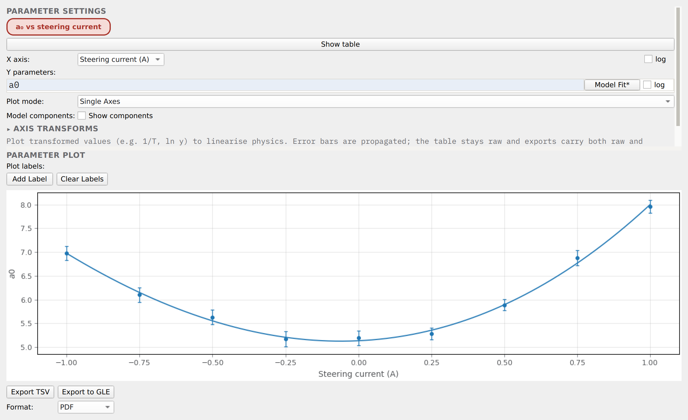
The Fit Parameters panel plotting the Ag-mask initial asymmetry \(a_0\) against Steering current (A) — the manual column, chosen on the X axis selector. The nine per-run \(a_0\) values rise from ≈ 7 % at ±1 A to a shallow minimum near zero, and a Model Fit cubic is overlaid on the points. The fitted minimum falls at \(I = -0.060\) A: with the beam centred, muons pass through the Ag aperture onto the depolarising Fe₂O₃, so the Ag-mask signal is lowest at the centred current. That reproduces the WiMDA-graded muon-school answer for this exercise — a beam-centred steering current of essentially 0 A.

A Cubic model is used, rather than a plain parabola, because the WiMDA reference curve is itself a cubic; its minimum at \(I = -0.060\) A is the graded deliverable. The same panel exports the trend (Export TSV, Export to GLE) once you are happy with it.

Reusing the calibration

When you load further runs of the same instrument, Asymmetry auto-applies the active profile to them (the Log shows “Auto-applied existing project grouping”) so a whole series inherits the same \(F\)/\(B\) split, dead-time mode, and good-data window with no per-run Apply step. The measured per-run quantities — good-frame counts, \(t_0\) — are always re-read from each run, never inherited.

\(\alpha\), however, is a sample calibration, not an instrument constant. Every run inheriting the profile carries its \(\alpha\), so when you switch to a new sample, start a new profile for that sample and re-Calibrate α from a reference run before trusting the asymmetry. If one run in a series genuinely needs its own grouping — a masked detector, say — use the scope panel’s Release from profile button rather than starting a new profile for the whole series. A finished profile is saved with the project, so it is ready to reuse the next time that project is opened.

Where to go next

• Detector Grouping and Layout — full grouping-profile and layout-editor reference.

• Grouping and calibration walkthrough — a second worked calibration walkthrough, plus the scriptable API.

• Temperature scan through a magnetic transition — applies one calibrated profile across a temperature scan.

• Muon diffusion in copper: Kubo–Toyabe, Abragam, and QLCR — uses this setup as the front end to a zero-field dynamics fit.

References

• Kilcoyne, RAL Report RAL-94-080 (1994) — per-detector dead-time determination from a silver sample.