Muon diffusion in copper: Kubo–Toyabe, Abragam, and QLCR

Copper is the textbook host for muon diffusion. A positive muon stops at an octahedral interstitial site in the face-centred-cubic lattice, where it behaves as a light isotope of hydrogen — a proton with one ninth of the mass — and its spin dephases in the static dipolar field of the surrounding ⁶³Cu and ⁶⁵Cu nuclear moments. As the sample warms the muon begins to hop between sites, the field it samples fluctuates, and the relaxation motionally narrows. Copper is the classic choice precisely because hydrogen itself is too insoluble in the metal to study by conventional means, so the muon stands in for it. Tracking how the relaxation changes with temperature turns a µSR spectrometer into a diffusion probe.

This worked example follows the WiMDA muon-school copper set through the three field geometries the guide prescribes, using real corpus data at every step:

• zero field (ZF) — the static Gaussian Kubo–Toyabe dip at 40 K, and its departure at base temperature that signals low-temperature quantum diffusion;

• zero field, warmed — the dynamic Kubo–Toyabe fit that extracts the hop rate \(\nu(T)\), whose temperature dependence resolves a mobility minimum and an activation energy;

• transverse field (TF) — the Abragam line shape that measures the same hop rate a second way, as an independent cross-check;

• longitudinal field (LF) — the quadrupolar level-crossing resonance (QLCR), a resonance unique to the muon sitting next to a quadrupolar nucleus.

The experiment and the corpus data

The corpus example (Nuclear magnetism and ionic motion → Muon diffusion and QLCR in copper, Data/) ships 74 NeXus .nxs runs from two campaigns: a 2010 EMU set (runs 20882–20917) and a 2024 ARGUS set (runs 76924–76961), both pulsed ISIS instruments. Between them they cover all three geometries.

Runs	Field / mode	Role in this workflow
20886 (40 K), 20887 (~5 K)	ZF	The static-KT signature and the low-temperature contrast that opens the quantum-diffusion question (EMU).
20886, 20901–20917 (+ 20887)	ZF, 5–200 K	The dense ZF temperature scan fitted with the dynamic Kubo–Toyabe to build \(\nu(T)\) (EMU).
20883–20885	TF 100 G	The transverse-field line shape, fitted with the Abragam envelope to cross-check the hop rate (EMU).
20888–20900	LF 40–120 G, 40 K	The quadrupolar level-crossing field scan, densely sampled around the resonance (EMU).
76935	ZF 40 K	The highest-statistics single 40 K run, used for the clean static-KT render (ARGUS).

Set up the detector grouping as in EMU detector grouping and α calibration — the EMU Longitudinal preset for the ZF and LF runs; \(\alpha\) is not critical for a ZF relaxation shape but matters for the TF precession amplitude. The EMU loader reads each run’s applied field and setpoint temperature from the file header, so the B (G) and T (K) columns of the Data Browser are populated automatically — the field axis of the QLCR scan below comes straight from that metadata.

The static Kubo–Toyabe signature

At 40 K the muon is effectively static on the µSR timescale: it sits in one interstitial site for far longer than the microseconds over which its spin relaxes. A static, dense, isotropic distribution of local fields produces the static Gaussian Kubo–Toyabe relaxation, whose zero-field shape is unmistakable — an early Gaussian dip to a minimum, a partial recovery, and then a flat tail at one third of the initial asymmetry. The ⅓ tail is the zero-field fingerprint of static disorder: one third of the muons find their local field pointing along their initial spin and do not depolarise.

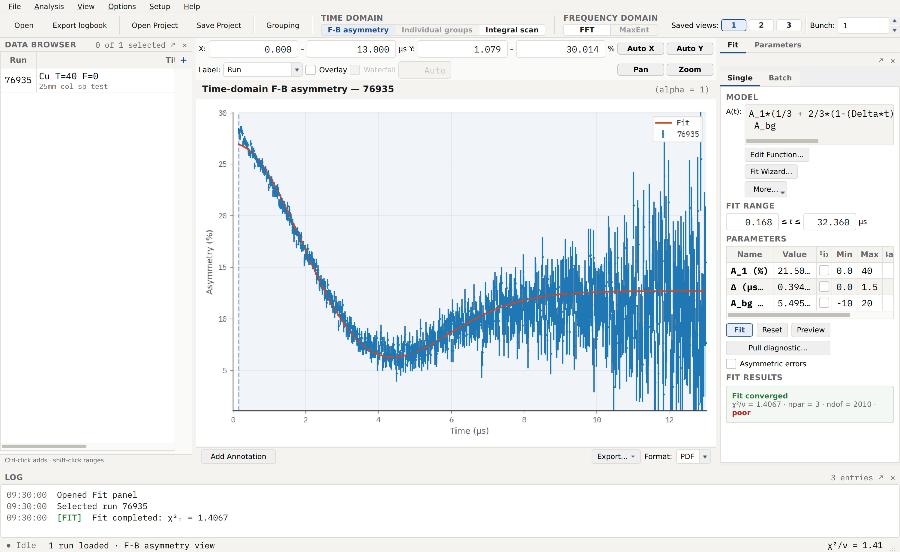
The StaticGKT_ZF + Constant fit to the ARGUS 40 K zero-field run 76935 in the Single fit tab. The red Fit curve traces the Gaussian dip to its minimum near 4.5 µs and the recovery to the flat ⅓ tail — the signature static Kubo–Toyabe. The PARAMETERS table reports \(A_1 = 21.5\) %, a static width \(\Delta = 0.394\) µs⁻¹, and a background \(A_{bg} = 5.5\) %. That width lands squarely on the literature anchor for octahedral muons in copper, \(\Delta \approx 0.38\)–\(0.39\) µs⁻¹. The FIT RESULTS badge reads poor at \(\chi^2/\nu = 1.41\) (npar = 3, ndof = 2010): the badge applies a strict threshold, but the fit is visually excellent over the whole window. The view is framed to the first 13 µs because past there the zero-field forward/backward asymmetry ratio diverges as its denominator runs down — the noise fan filling the right of the panel.

The width \(\Delta\) is a property of the lattice — the geometry and magnitude of the ⁶³Cu/⁶⁵Cu dipolar fields at the muon site — not of temperature, so it serves as a fixed anchor for the dynamic fits that follow. The corpus teaching guide states no target value for it; the \(0.38\)–\(0.39\) µs⁻¹ figure is a literature sanity anchor (a zero-field measurement gives \(0.389(3)\) µs⁻¹), used here only to confirm the fit is physical.

The static Gaussian Kubo–Toyabe function

For a static, isotropic Gaussian distribution of local fields with root-mean-square width \(\Delta/\gamma_\mu\) along each axis, the zero-field muon polarisation is

\[G^{\mathrm{stat}}_{\mathrm{KT}}(t) = \frac{1}{3} + \frac{2}{3}\,(1 - \Delta^2 t^2)\,\exp\!\left(-\tfrac{1}{2}\Delta^2 t^2\right).\]

The \(\tfrac{2}{3}\) transverse component gives the Gaussian dip and recovery; the \(\tfrac{1}{3}\) longitudinal component is the flat tail. The full component, its longitudinal-field generalisation, and the relation \(\sigma = \Delta/\sqrt{2}\) are on the Kubo–Toyabe reference page.

Low-temperature quantum diffusion

The guide poses two linked questions: at 40 K, is the zero-field relaxation the signature Kubo–Toyabe you expect? And at base temperature, how does the spectrum differ — and why? Overlaying the two ZF runs answers both at once.

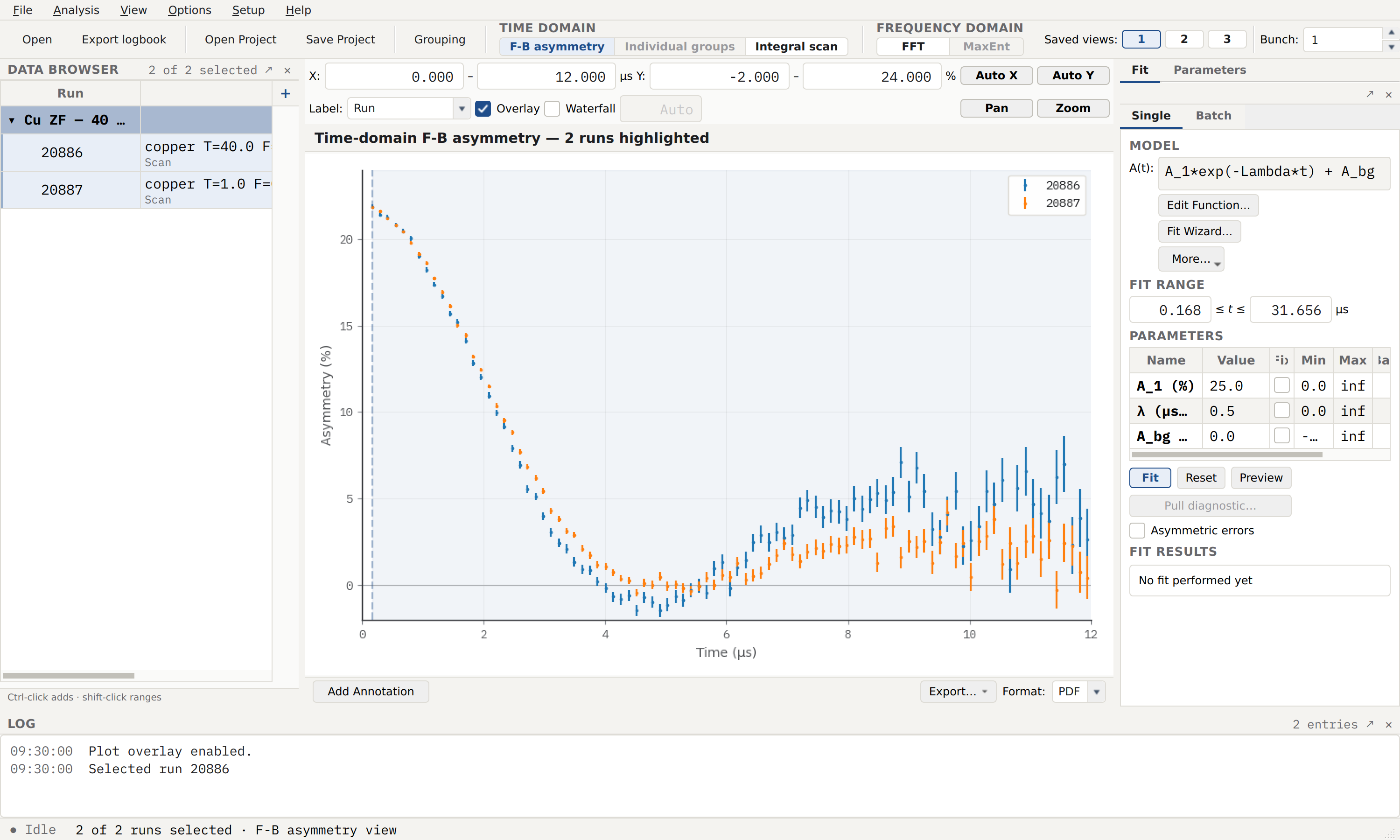
The EMU zero-field runs 20886 (40 K, blue) and 20887 (~5 K, orange) loaded into one data group and drawn with Overlay enabled, the bins bunched 8× so the late-time contrast reads through the zero-field noise. The early-time Kubo–Toyabe dip is common to both — the field-width the muon sees is temperature-independent. The difference is in the tail: at 40 K (blue) the polarisation recovers to a flat ⅓ plateau, the static-KT expectation; at ~5 K (orange) that tail relaxes further, drifting below the 40 K trace past about 6 µs.

A relaxing ⅓ tail is the tell-tale of a field that is not quite static: the distribution is being partly averaged by motion. The counter-intuitive part is that this happens on cooling. Classically the muon should freeze ever more firmly into its site as thermal energy is removed, and the tail should become more flat, not less. Instead the hop rate turns back up at low temperature — the muon delocalises and moves by coherent quantum tunnelling rather than by thermal activation over the site-to-site barrier. This is the low-temperature branch of quantum diffusion, seen directly in copper by Luke et al., Phys. Rev. B 43, 3284 (1991), who tracked the hop rate rising again below ~1 K while the static width stayed fixed at \(\approx 0.39\) µs⁻¹.

Note

The base-temperature run 20887 is set to 1 K but its thermometer reads 5.8 K (a known low-temperature read-back artefact); either way it is the coldest, most weakly dynamic point in the ZF series, and the qualitative story — a relaxing ⅓ tail below the static-KT plateau — is unchanged.

The dynamic Kubo–Toyabe fit and the hop rate

Between the static 40 K limit and the fast-hopping high-temperature limit, the relaxation is described by the dynamic Gaussian Kubo–Toyabe function. It is the strong-collision generalisation of the static form: a muon samples one field from the Gaussian distribution, then at random intervals set by the fluctuation rate \(\nu\) jumps to a fresh, uncorrelated field. As \(\nu\) rises the Kubo–Toyabe minimum fills in and the ⅓ tail lifts and then relaxes; once \(\nu \gg \Delta\) the relaxation motionally narrows toward a simple exponential \(\exp(-2\Delta^2 t/\nu)\). The rate \(\nu\) is the muon hop rate, so fitting it at each temperature is the measurement.

Use DynamicGaussianKT (composited with a flat Constant background). The parameters are the amplitude A_1 (%), the static width Delta (\(\mu\mathrm{s}^{-1}\)), the fluctuation rate nu (MHz), a longitudinal field B_L (G) held at zero, and the background A_bg (%). Two settings matter:

• Fix B_L = 0. The runs are zero-field; the ⅓ tail belongs to the KT function itself, and a spurious field would compete with it.

• Fix Delta at its static value (0.37–0.39 µs⁻¹ from the low-temperature reference) and float nu — because \(\Delta\) and \(\nu\) are strongly correlated and floating both is degenerate, the fit trading width against rate at essentially the same \(\chi^2\).

Parameter	Seed	Setting	Meaning
A_1 (%)	20	free	Asymmetry amplitude
Delta (µs⁻¹)	0.37	fixed	Static Gaussian width, from the low-\(T\) reference
nu (MHz)	1.0	free	Field-fluctuation / hop rate — the quantity of interest
B_L (G)	0.0	fixed	Longitudinal field, zero here
A_bg (%)	0.0	free	Flat background

Taking the warmest EMU run 20917 (200 K) as a worked single fit:

from asymmetry.core.io import load
from asymmetry.core.fitting.engine import FitEngine
from asymmetry.core.fitting.models import MODELS
from asymmetry.core.fitting.parameters import Parameter, ParameterSet

ds = load(".../Muon diffusion and QLCR in copper/Data/EMU00020917.nxs")

model = MODELS["DynamicGaussianKT"]
params = ParameterSet([
    Parameter("A0", value=20.0, min=0.0),
    Parameter("Delta", value=0.37, fixed=True),   # static width, held
    Parameter("nu", value=1.0, min=0.0),           # the parameter of interest
    Parameter("B_L", value=0.0, fixed=True),
    Parameter("baseline", value=0.0, fixed=True),  # ZF: no free offset
])
result = FitEngine().fit(ds, model.function, params)

fitted = {p.name: p.value for p in result.parameters}
print(round(fitted["nu"], 2))                       # 2.40 (MHz)

The fit converges with \(A_0 \approx 21.7\,\%\) and

\[\nu \approx 2.40\;\mathrm{MHz} \quad (\text{reduced } \chi^2 \approx 0.94),\]

a clear sign the muon is hopping rapidly at 200 K. Releasing \(\Delta\) lands at \(\Delta \approx 0.31\;\mu\mathrm{s}^{-1}\), \(\nu \approx 1.6\;\mathrm{MHz}\) at the same \(\chi^2\) — the \(\Delta\)–\(\nu\) degeneracy that motivates holding \(\Delta\) fixed.

The hop-rate curve and the mobility minimum

Repeating the dynamic-KT fit across the ZF temperature scan — warm-starting each temperature from the previous fit’s converged values, the guide’s “follow the relaxation up in temperature” recipe — builds the hop rate \(\nu(T)\). This is the headline result of the whole example, and it is not a simple straight line: the hop rate spans two decades and turns over.

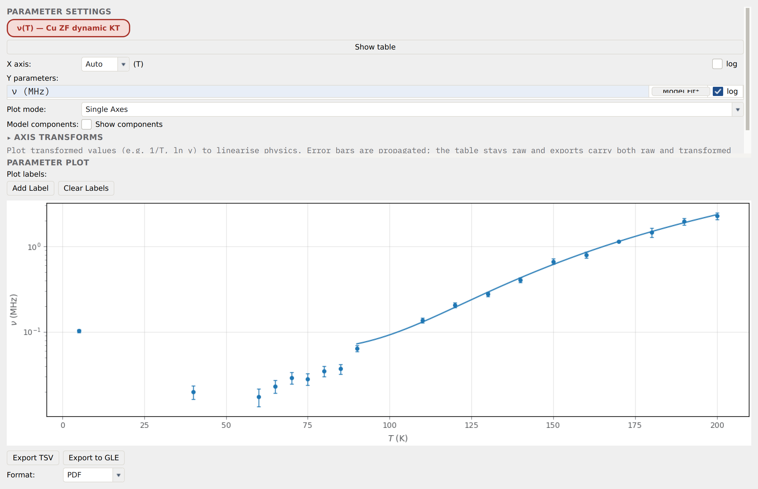
The \(\nu(T)\) trend in the parameter-trending panel, with the log toggle on the \(\nu\) axis enabled so the two-decade span reads in one frame. The rate falls from \(\approx 0.10\) MHz at ~5 K to a minimum of \(\approx 0.02\) MHz near 60 K — the mobility minimum — and then climbs steeply to \(\approx 2.3\) MHz at 200 K. The blue curve is a Model Fit* of an Arrhenius + Constant model over the thermally activated \(T \ge 90\) K branch; its slope gives the activation energy.

Two regimes meet at the minimum. Above it, hopping is thermally activated — the muon climbs over the site-to-site barrier, and the rate follows an Arrhenius law \(\nu(T) = a\,e^{-E_a/k_B T} + c\). Below it, the rate turns up again on cooling: this is the low-temperature quantum-diffusion branch seen in the 5 K vs 40 K contrast above. Fitting the activated branch (\(T \ge 90\) K) with an Arrhenius + Constant model gives

\[E_a \approx 73\;\mathrm{meV},\]

in the expected range for muon diffusion in copper. The value is window-dependent — it drifts with where the low-temperature end of the branch is cut — and a narrower or wider fit range shifts it by several meV; the corpus program’s own run gave \(E_a \approx 62\) meV over a slightly different window. Both describe the same over-barrier hopping.

Warning

The low-temperature upturn is resolved but not fully mapped. There is only one sub-40 K zero-field run per instrument (EMU 20887 at ~5 K) and no sub-kelvin data, so the mobility minimum is clear — the ~5 K rate (\(\approx 0.10\) MHz) sits well above the ~60 K minimum (\(\approx 0.02\) MHz) — but the full coherent-tunnelling upturn that Luke et al. traced below ~1 K is out of range. Read the low-T side as “minimum plus a single elevated point”, not as a complete quantum-diffusion curve.

Cross-check: the transverse-field Abragam line shape

The same hop rate can be measured a second, independent way, in transverse field. Applying a field perpendicular to the initial muon spin makes the muons precess at their Larmor frequency \(f = \gamma_\mu B\) (\(\gamma_\mu = 135.5\) MHz T⁻¹); the nuclear-dipolar dephasing then shows up as a damping envelope on the precession. As the muon starts to hop, that envelope changes shape — Gaussian at low temperature where the field is static, crossing over to exponential at high temperature as motion narrows it. The Abragam relaxation function is exactly this Gaussian-to-exponential crossover envelope, carrying the same \(\Delta\) and \(\nu\) as the Kubo–Toyabe family. Building the model as the multiplicative composite Oscillatory × Abragam + Constant gives the assembled form

A(t): A_1*cos(2*pi*f*t + phi) * G_Abragam(Delta, nu) + A_bg

— a precession damped by the Abragam envelope, with a flat background. Asymmetry de-duplicates the shared amplitude and baseline of the two multiplied components, so the composite collapses to a single amplitude \(A_1\cos(2\pi f t + \varphi)\,G_{\mathrm{Abragam}}(\Delta,\nu)\) plus A_bg.

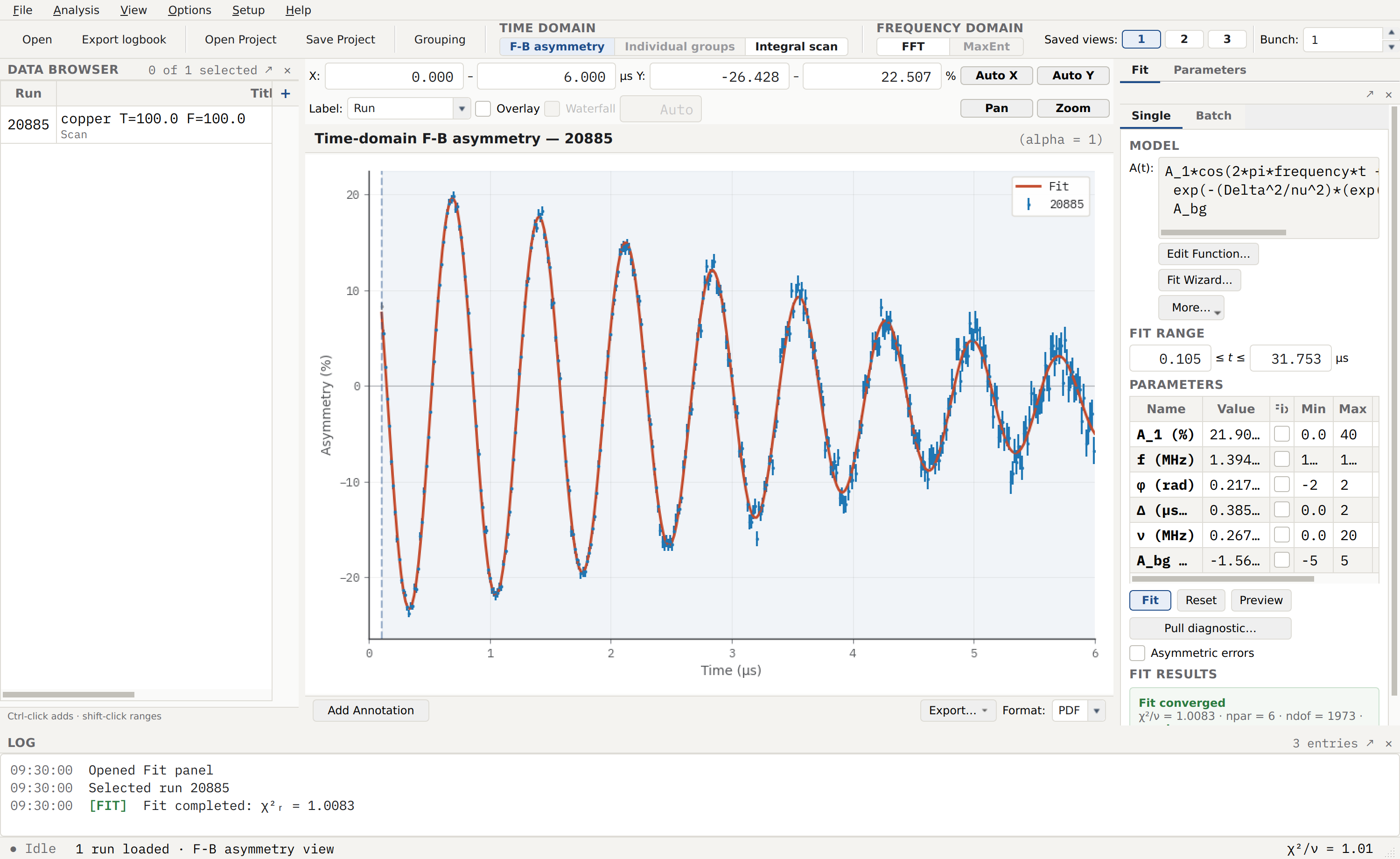
The Oscillatory × Abragam + Constant fit to the EMU 100 G transverse-field run 20885 (100 K), framed to the first 6 µs so the ~1.4 MHz precession and its damping envelope are both resolved. The PARAMETERS table reports \(f = 1.395\) MHz (the expected Larmor frequency at 100 G), \(\varphi = 0.22\) rad, a width \(\Delta = 0.385\) µs⁻¹, and a hop rate \(\nu = 0.267\) MHz, with \(\chi^2/\nu = 1.01\). The fitted \(\Delta = 0.385\) µs⁻¹ cross-checks the zero-field static width to within a few percent — the same nuclear-dipolar distribution, seen in a different geometry — and the transverse-field hop rate is consistent with the ZF dynamic-KT rate at the same temperature, the consistency the guide asks for.

Quadrupolar level-crossing resonance (QLCR)

The longitudinal-field runs probe a different piece of physics entirely. The positive muon distorts its interstitial cage and sets up an electric-field gradient at the neighbouring Cu nuclei; those nuclei (spin \(I = 3/2\)) carry an electric quadrupole moment, so the field gradient splits their spin levels. In an applied longitudinal field the muon Zeeman levels and these quadrupolar-split nuclear levels shift at different rates, and at one particular field they cross. The muon–nucleus dipolar coupling turns the crossing into an avoided crossing: muon and nuclear spin become resonantly mixed, opening a fast relaxation channel. The result is a quadrupolar level-crossing resonance (QLCR) — a dip in the time-integrated muon asymmetry as the field is stepped through the crossing.

Asymmetry analyses this by integral counting, in the Integral scan (ALC) representation. Rather than fit a model to each spectrum, it reduces every run to one number — the asymmetry integrated over a fixed time window — and plots that against the swept field. A resonance shifts the time-averaged asymmetry, so it appears directly as a feature in \(A\) versus field.

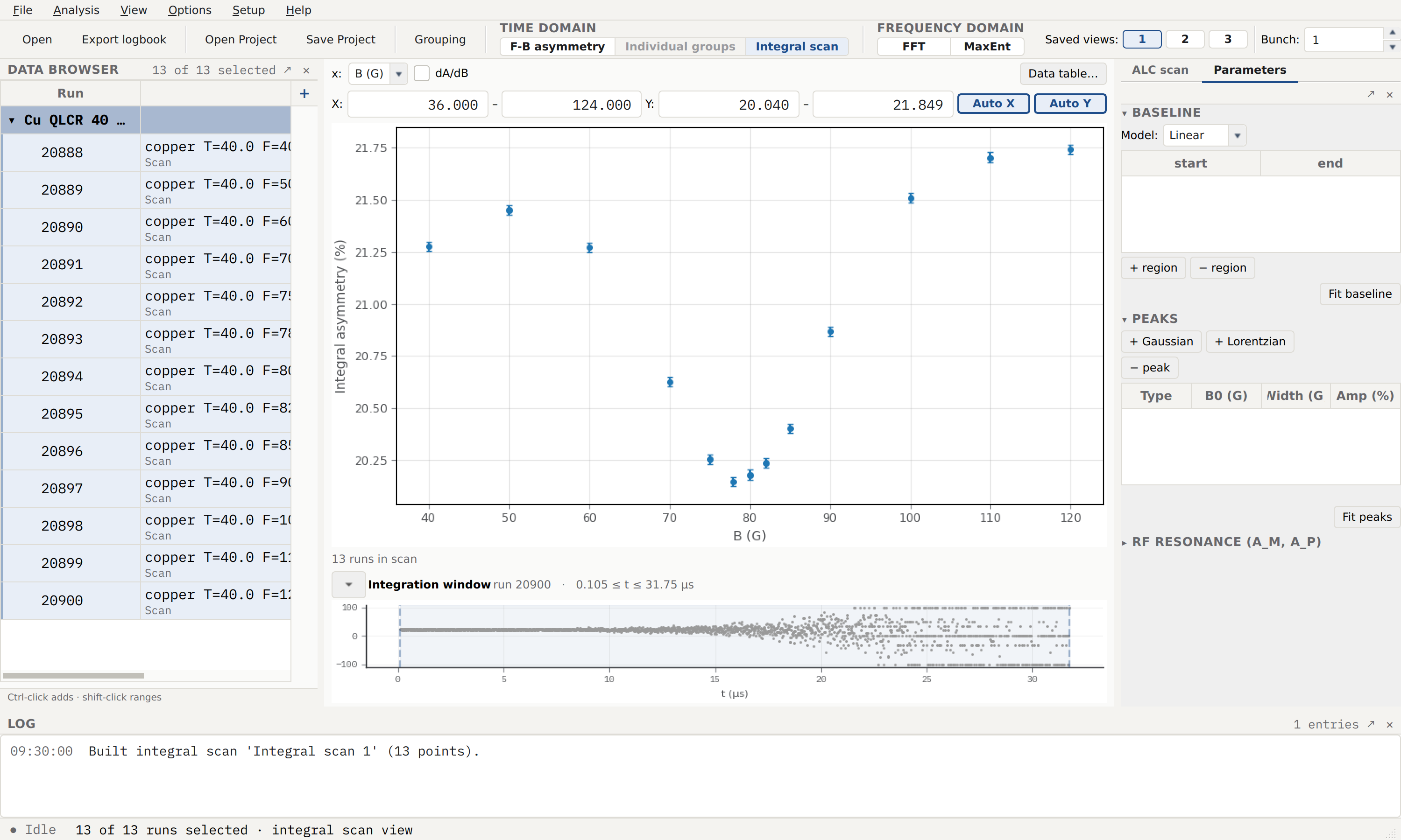
The QLCR field scan: the 13 EMU 40 K longitudinal-field runs 20888– 20900 reduced to one integral-asymmetry value each and plotted against the B (G) field axis in the Integral scan view. The scan dips to a clear minimum near 78 G — the level-crossing field — on a gently rising baseline, the reason the BASELINE model is set to Linear. The slim Integration window strip beneath the scan shows the 0.1–31.75 µs window over which each run was integrated, and the Parameters dock carries the BASELINE, PEAKS (+ Gaussian / + Lorentzian), and RF RESONANCE (A_M, A_P) sections used to fit the dip. The densest sampling sits at 75–90 G, deliberately concentrated to pin the resonance field.

The corpus guide states no expected resonance field; it is a deliverable, to be located from the dip. The dense 75–90 G sampling and the minimum near 78 G are consistent with the known copper QLCR, first reported by Kreitzman et al., Phys. Rev. Lett. 56, 181 (1986). The same resonance can also be extracted by fitting a longitudinal-field relaxation function to each spectrum and plotting the rate against field — where the integral dip becomes a rate peak — the second method the guide names.

The level-crossing condition

A level crossing occurs when the muon Zeeman splitting matches an energy gap of the coupled muon–nucleus system:

\[\hbar\,\gamma_\mu B_{\mathrm{res}} \approx \Delta E_{\mu\text{-}N},\]

where \(\Delta E_{\mu\text{-}N}\) is set by the nuclear quadrupole coupling (the electric-field gradient the muon induces at the Cu site) and, more weakly, by the muon–nucleus dipolar interaction that mixes the states and gives the resonance its width. Because the gap is fixed by the local electronic and lattice environment, the resonance field \(B_{\mathrm{res}}\) is a fingerprint of the muon site and its neighbours; its temperature and motional narrowing report on muon dynamics near the site. See Integral scan mode (avoided-level-crossing field scans) for the integral-asymmetry observable and the baseline/peak fitting workflow, and Kreitzman et al. for the copper-specific analysis.

Assumptions and limitations

• Δ is anchored, not measured per run. The dynamic-KT hop rate depends on holding \(\Delta\) fixed at its static value; \(\Delta\) and \(\nu\) are degenerate in a single spectrum. The static width is taken from the low-temperature ZF fit (0.37–0.39 µs⁻¹), and the extracted \(\nu\) inherits any error in that anchor. Above ~100 K a free-\(\Delta\) fit drifts lower (motional narrowing), which is expected but also a reminder that the fixed value is an approximation there.

• The activation energy is window-dependent. \(E_a \approx 73\) meV comes from an Arrhenius fit to the \(T \ge 90\) K branch; a different low-T cut-off shifts it by several meV (the corpus program obtained ~62 meV over a nearby window). Quote it with the fit window, not as a hard number, and note the guide states no target value — \(E_a\) is a deliverable.

• The low-temperature quantum-diffusion branch is under-sampled. With one sub-40 K ZF run and no sub-kelvin data, the mobility minimum resolves but the coherent-tunnelling upturn is not mapped. The 5 K point also carries a thermometer read-back ambiguity (set 1 K, read 5.8 K).

• The QLCR resonance field is read off the scan, not fitted here. The integral-counting dip locates the resonance near 78 G; a baseline-plus-peak fit (or the relaxation-rate method) would return a resonance field and width with uncertainties. The scan also rides a sloping baseline, so a Linear baseline must be fitted before the dip depth is meaningful.

• ν units carry a 2π ambiguity. Fluctuation rates in the Kubo–Toyabe and Abragam parameterisations are variously quoted in MHz or in angular µs⁻¹, which differ by \(2\pi\). The values here follow the program’s convention as displayed; do not assume a conversion when comparing across sources.

References

• R. S. Hayano, Y. J. Uemura, J. Imazato, N. Nishida, T. Yamazaki, and R. Kubo, Phys. Rev. B 20, 850 (1979) — the dynamic Kubo–Toyabe strong-collision theory used for the ZF hop-rate fits.

• R. Kubo and T. Toyabe, in Magnetic Resonance and Relaxation, edited by R. Blinc (North-Holland, Amsterdam, 1967), p. 810 — the original Kubo–Toyabe zero-field relaxation function.

• A. Abragam, The Principles of Nuclear Magnetism (Oxford University Press, Oxford, 1961) — the Gaussian-to-exponential crossover envelope used on the transverse-field line shape.

• G. M. Luke, J. H. Brewer, S. R. Kreitzman, D. R. Noakes, M. Celio, R. Kadono, and E. J. Ansaldo, Phys. Rev. B 43, 3284 (1991) — muon diffusion and spin dynamics in copper, including the low-temperature quantum-diffusion upturn.

• S. R. Kreitzman, J. H. Brewer, D. R. Harshman, R. Keitel, and D. Ll. Williams, Phys. Rev. Lett. 56, 181 (1986) — the quadrupolar level-crossing resonance of the muon in copper.

• S. J. Blundell, R. De Renzi, T. Lancaster, and F. L. Pratt, Muon Spectroscopy: An Introduction (Oxford University Press, Oxford, 2022), Ch. 5–6 — Kubo–Toyabe relaxation, dynamics, and level-crossing resonance.

Cross-references

• EMU detector grouping and α calibration — the EMU grouping profile and α calibration that front-ends every fit here.

• StaticGKT_ZF — the static Gaussian Kubo–Toyabe reference, used to anchor \(\Delta\).

• DynamicGaussianKT — the dynamic Gaussian Kubo–Toyabe reference and its motional-narrowing limit.

• Abragam — the Abragam relaxation reference, the transverse-field crossover envelope.

• Integral scan mode (avoided-level-crossing field scans) — the Integral scan (ALC) mode used for the QLCR field scan.

• Parameter trending — the trending panel, log axes, and the Arrhenius-on-a-plateau recipe used for \(\nu(T)\).

• LF decoupling and static-vs-dynamic field distributions — the static-versus-dynamic Kubo–Toyabe formalism worked on a synthetic Ag decoupling series.

• Global fitting across fields: Li⁺ ionic motion in a garnet electrolyte — the same dynamic-relaxation trending workflow applied to Li⁺ ionic motion, via a global fit across fields.