LF decoupling and static-vs-dynamic field distributions

A longitudinal-field (LF) decoupling series answers one question: are the local fields the muon senses static or dynamic? The two cases look almost identical in a single zero-field spectrum, yet they demand different models and carry different physics. Decoupling separates them. In a static distribution the polarisation is fully recovered once the applied field exceeds the internal width, and the relaxation switches off at a fixed field. In a dynamic distribution the relaxation survives to high field and its rate falls smoothly as \(1/B^2\) — the Redfield signature — so a field scan measures both the field width and the fluctuation time.

This chapter works the dynamic case on real data: the Ca₃Co₂O₆ magnetic-plateau decoupling scan from the WiMDA muon school corpus (HiFi runs 9023–9051, 15 K, 0–3.8 T), the same measurement published by Baker, Lord, and Prabhakaran, J. Phys.: Condens. Matter 23, 306001 (2011). Its headline is the Redfield linearisation — \(1/\lambda\) against \(B^2\) — built directly in the parameter-trending panel using the native axis transforms (Parameter trending), so the paper’s Fig. 2(b) is reproduced without leaving the GUI. A short contrast section then shows the static counter-example on the superconductor Re₆Zr, where 10 mT of longitudinal field fully decouples a static Gaussian Kubo–Toyabe relaxation — the discriminating diagnostic in its cleanest form.

Physical motivation

A muon implanted in a magnetic material samples a distribution of local fields \(B_\mu\). The relaxation of its spin polarisation depends both on the width of that distribution and on whether the fields are frozen on the muon’s observation timescale (~10 µs) or fluctuating.

For a static isotropic distribution of width \(\Delta/\gamma_\mu\), the zero-field polarisation is the static Gaussian Kubo–Toyabe function

\[P_z^{\mathrm{KT}}(t) = \frac{1}{3} + \frac{2}{3} (1 - \Delta^2 t^2)\exp\!\left(-\frac{\Delta^2 t^2}{2}\right),\]

whose long-time recovery to one-third of the initial polarisation — the “1/3 tail” — is the fingerprint of an isotropic static field. Applying a longitudinal field \(B_L\) quenches the perpendicular dephasing once \(\gamma_\mu B_L \gg \Delta\), and the polarisation is decoupled back to unity. The field needed is set only by the static width, so decoupling happens abruptly over a narrow field range.

If the fields fluctuate with a single correlation time \(\tau\), the static formula no longer holds. In the motionally-narrowed limit the relaxation is a single exponential, \(P_z(t) = \exp(-\lambda t)\), and its rate obeys Redfield’s equation

\[\lambda(B_L) = \frac{2\gamma_\mu^2 \Delta^2 \tau}{1 + \gamma_\mu^2 B_L^2 \tau^2},\]

with \(\gamma_\mu = 2\pi \times 135.5\;\mathrm{MHz\,T^{-1}}\). Here \(\Delta\) is the width of the fluctuating field distribution and \(\tau\) its correlation time. The decisive difference from the static case is that \(\lambda\) does not switch off at a threshold field: it falls continuously, as \(1/B_L^2\) once \(\gamma_\mu B_L \tau \gg 1\), and a scan of \(\lambda(B_L)\) measures \(\Delta\) and \(\tau\) separately.

Ca₃Co₂O₆ is a frustrated Ising-chain magnet: ferromagnetic Ising chains couple antiferromagnetically on a triangular lattice, and below \(T_{N1} = 25\) K the material develops a partial magnetisation plateau at one-third of saturation over the field range 0.5–3.6 T. Inside that plateau the internal fields are neither fully frozen nor fully paramagnetic — they fluctuate slowly, and the muon decoupling scan at 15 K is designed to catch them.

The data

The corpus holds the real HiFi ISIS NeXus (HDF4) files, runs 9023–9051, read natively by Asymmetry. Run 9023 is a TF20 calibration (300 K, 20 G transverse) that fixes \(\alpha\) and the field dependence of the initial asymmetry; the 15 K longitudinal-field scan runs from 9031 (zero field) to 9051 (3.8 T), stepping the applied field through and beyond the plateau. Ten million decay positrons were collected per run. The applied field is longitudinal throughout, so this is a decoupling scan, not a transverse-field precession measurement.

Two features of the raw data shape the analysis. First, below about 0.2 T the relaxation is faster than the ISIS pulse width can resolve and the observed asymmetry is suppressed, so the zero-field and 0.1 T runs cannot yield a physical \(\lambda\) and are excluded from the trend. Second, the initial asymmetry is only fully recovered by ~0.5 T; the constant background grows with field as decay positrons spiral in the applied field (from ~7 % at 1 T to ~37 % at 3.5 T), so every fit carries an additive background term.

Step 1 — Load and overlay the decoupling series

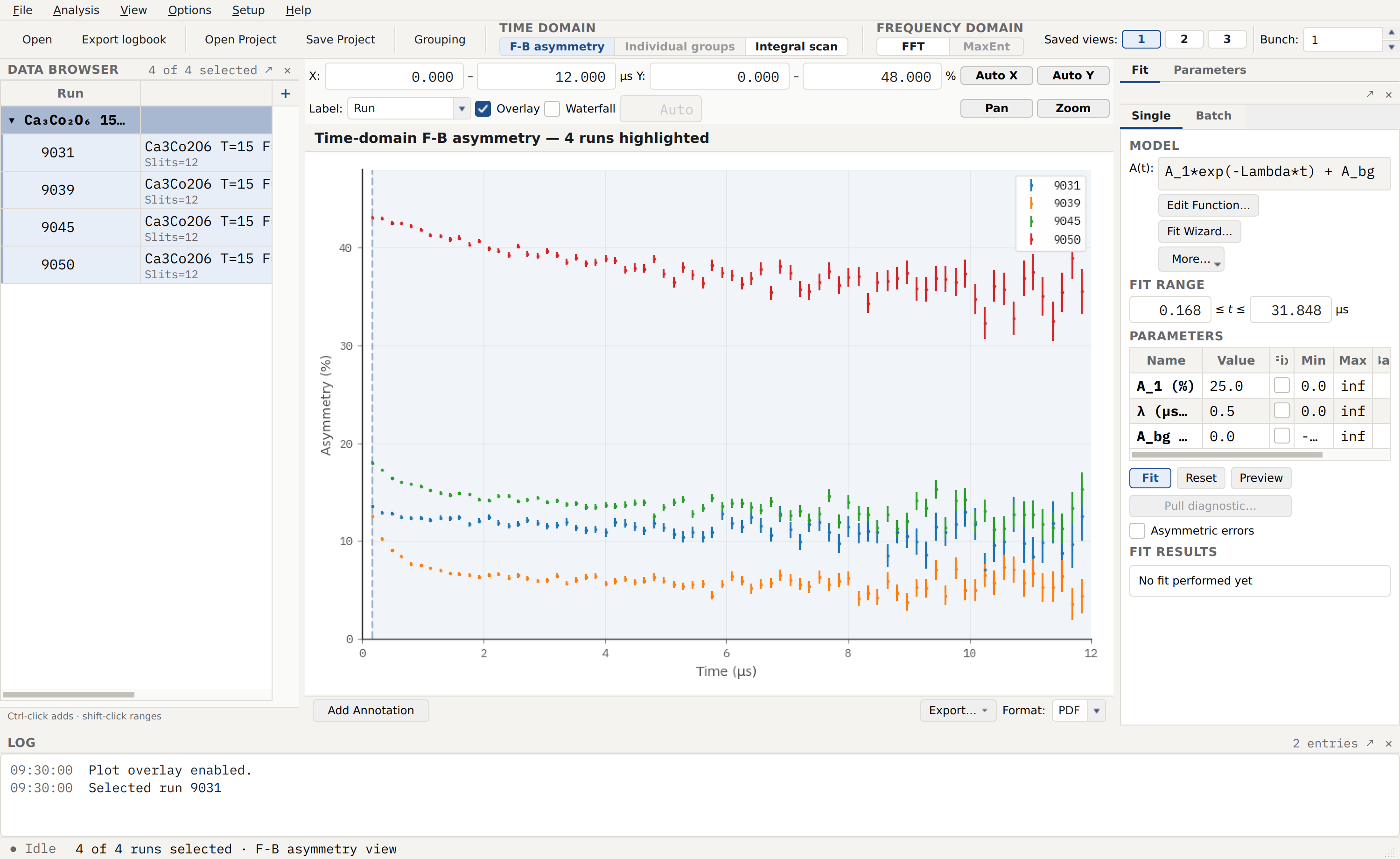
Four Ca₃Co₂O₆ 15 K LF spectra overlaid at zero field, 0.5, 1.5, and 3.5 T — Raw 15 K longitudinal-field spectra at zero field (9031), 0.5 T (9039), 1.5 T (9045), and 3.5 T (9050), loaded as the group `Ca₃Co₂O₆ 15 K LF scan` with **Overlay** enabled. The 3.5 T trace (red) is flat and high near 35–40 %: the muon is decoupled and the observed asymmetry has recovered. The lower-field traces relax within a few microseconds and sit lower, both because their relaxation is faster and because their recovered asymmetry is smaller. The vertical spread is therefore a mix of decoupling (flattening) and the field-dependent baseline.

Load the four representative runs and tick Overlay so all four draw on one set of axes. The qualitative decoupling picture reads straight off the plot: the relaxation flattens as the field rises. This is the same information the static case would give — a flat high-field trace — but here it is only the first half of the story. To tell dynamic from static we must measure how the rate falls with field, not merely that it falls.

Step 2 — Fit each run with a single exponential

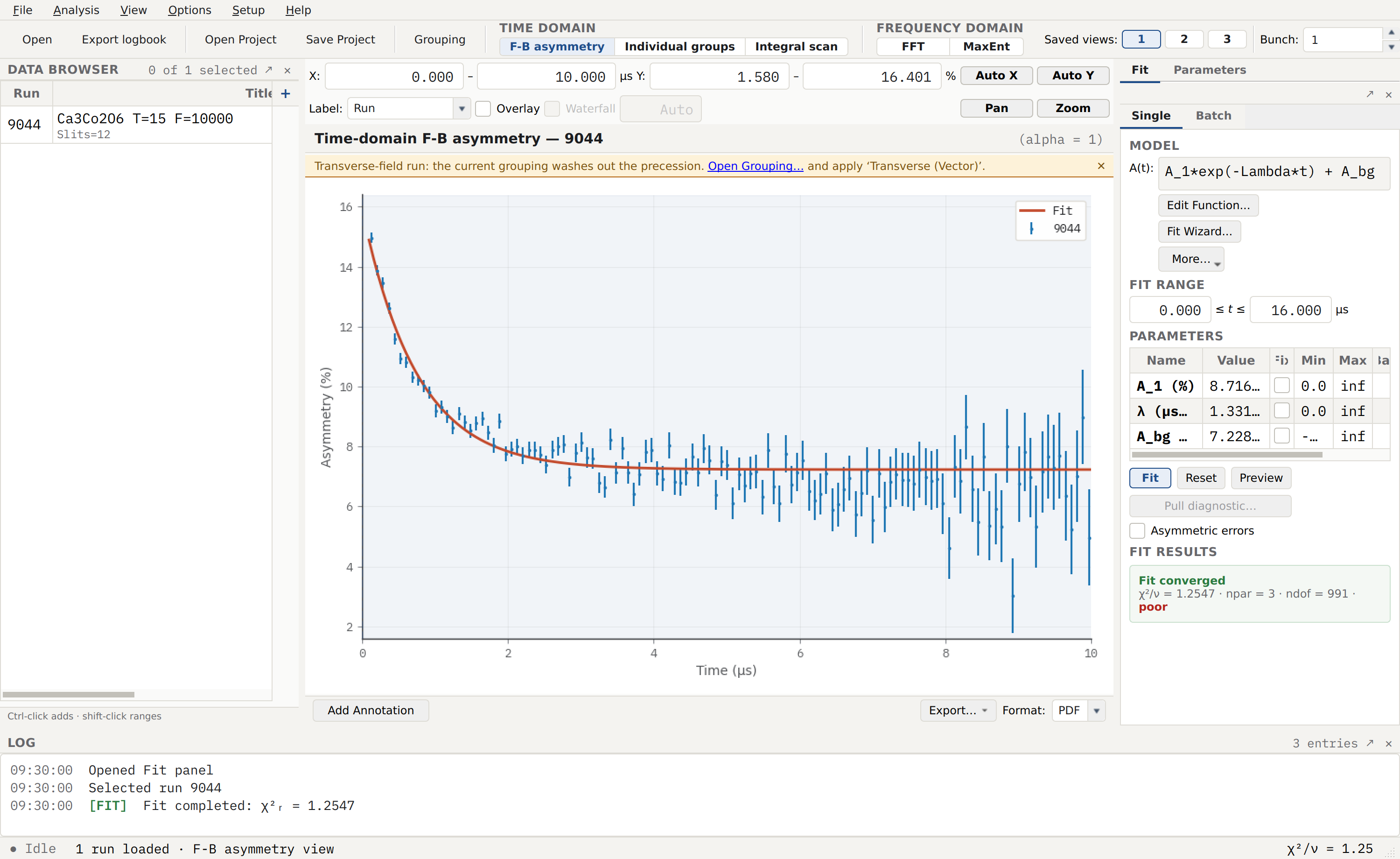
Converged Exponential + Constant fit on the Ca₃Co₂O₆ 1.0 T run 9044 — A converged `Exponential + Constant` fit on the 1.0 T run (9044), displayed bunched ×5 over 0–10 µs. The model line `A_1*exp(-Lambda*t) + A_bg` gives an initial asymmetry \(A_1 = 8.72\,\%\), a relaxation rate \(\lambda = 1.33\;\mu \mathrm{s}^{-1}\), and a background \(A_{bg} = 7.23\,\%\). The fit runs on the unbinned 0–16 µs data and converges cleanly.

The per-run model is Exponential + Constant, \(P_z(t) = A_1\,\exp(-\lambda t) + A_{bg}\), exactly the single exponential of the Redfield picture with an additive background. Seed \(\lambda\) high (~9 µs⁻¹) at low field and carry it downward from run to run in field order: the low-field runs are otherwise prone to walking into a spurious flat-line minimum. The additive \(A_{bg}\) absorbs the field-growing baseline from positron spiralling. Each converged run contributes one \(\lambda(B_L)\) point to the trend.

Note

The fit-results panel tags this fit’s \(\chi^2_r = 1.25\) (npar = 3, ndof = 991) with the wording poor. The verdict is the panel’s two-sided goodness-of-fit band (Parameter trending); with nearly a thousand degrees of freedom that band is narrow, and a \(\chi^2_r\) of 1.25 sits just outside it. The fit itself is good — the residual is the late-time forward–backward noise as the counts vanish, not a model deficiency.

Step 3 — Build the λ(B) trend

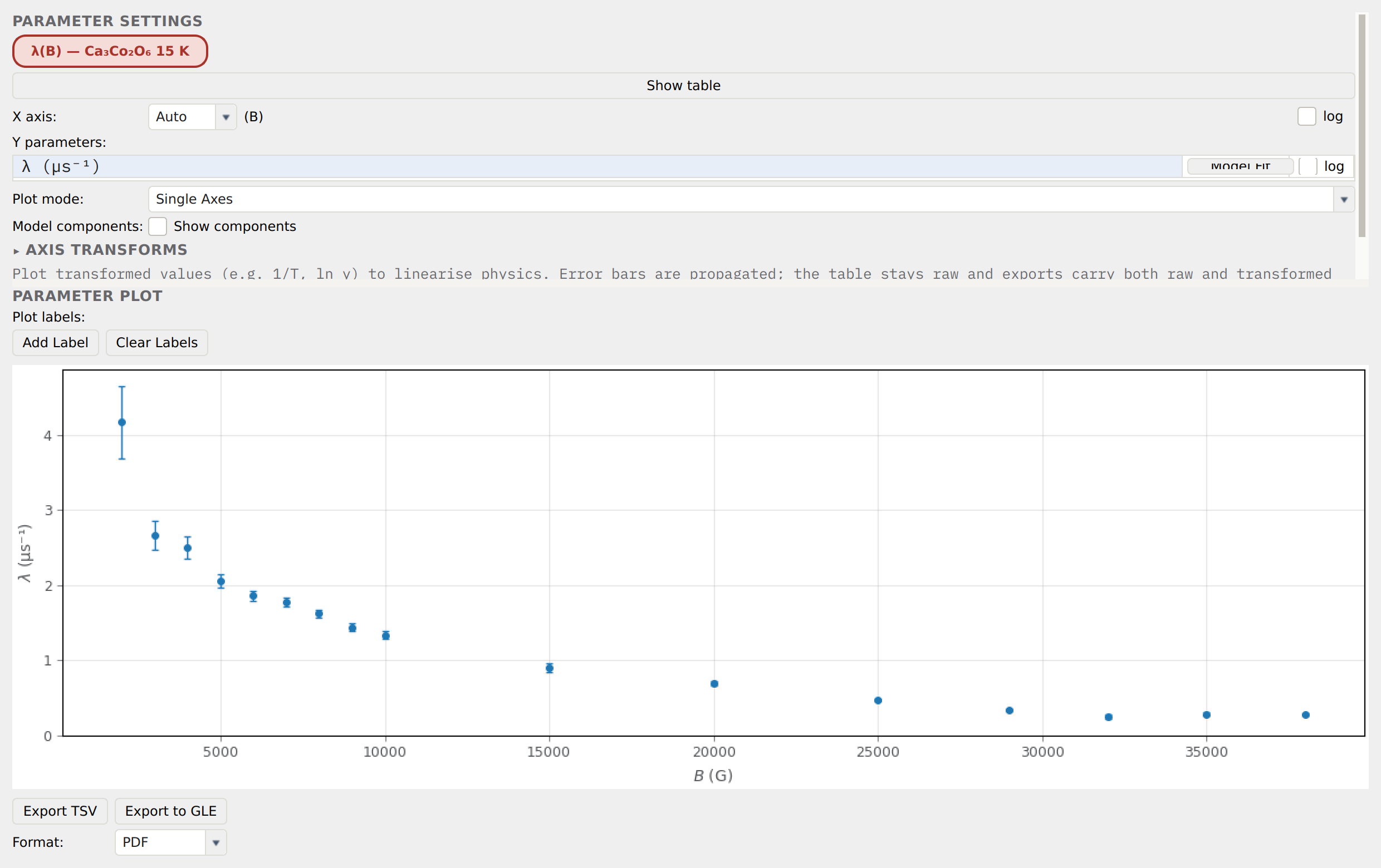
The relaxation rate lambda against applied field B for the Ca₃Co₂O₆ 15 K scan — The \(\lambda(B)\) trend in the parameter-trending panel (paper Fig. 2(a)), plotted on the panel’s native `B (G)` axis. The series is `λ(B) — Ca₃Co₂O₆ 15 K`; the y-parameter is `λ (µs⁻¹)`. The three regimes are visible: a rapid drop from ~4.2 µs⁻¹ at 0.2 T (2000 G), a slow decrease across the 0.5–3.6 T plateau, and a levelling to ~0.3 µs⁻¹ above 3.6 T.

Fitting every run from 0.2 T upward and collecting the rates builds the \(\lambda(B_L)\) curve. Its shape is the physics of the plateau. Below 0.5 T the bulk magnetisation is still rising and \(\lambda\) falls steeply; across the 0.5–3.6 T plateau it decreases slowly, the regime where the Redfield model holds; above 3.6 T the sample saturates into a field-polarised ferromagnet and \(\lambda\) is nearly constant. The zero- field and 0.1 T points are absent by design (Step 2): their relaxation is unresolvable at the ISIS pulse width, so they carry no physical rate.

That a dynamic rate should fall with field is already the qualitative discriminator. A static distribution would keep \(\lambda\) at its zero-field value until the decoupling threshold and then drop it to zero over a narrow range; a smooth \(1/B^2\)-like falloff spanning several tesla is the dynamic signature. The next step makes that quantitative.

Step 4 — The Redfield linearisation (headline)

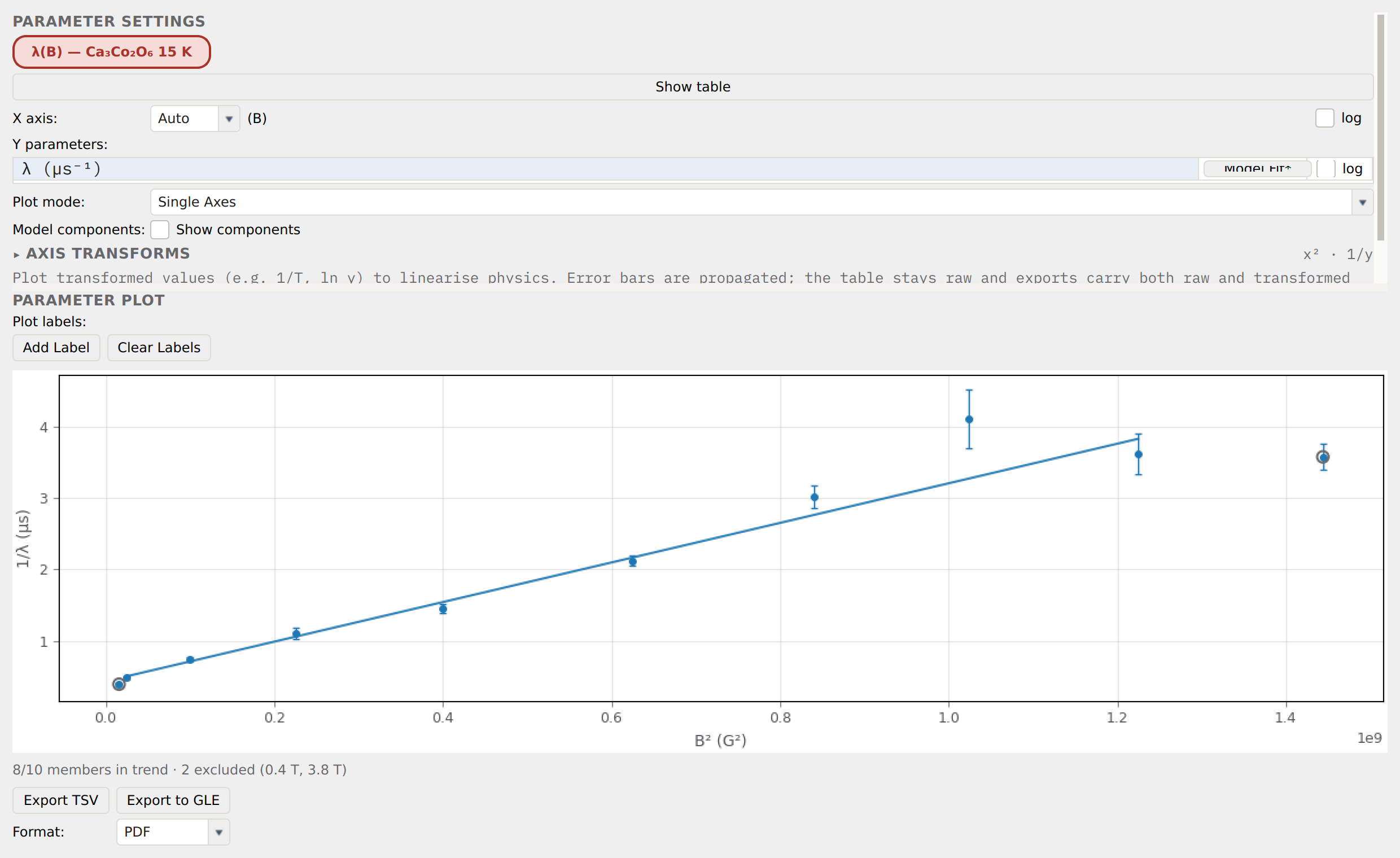
Redfield linearisation — 1/lambda against B squared with a linear fit over the plateau — The headline result: \(1/\lambda\) against \(B^2\) (paper Fig. 2(b)), built in the real trending panel with the **Axis transforms** set to `1/x (reciprocal)` on the Y axis and `x² (square)` on the X axis, and a `Linear` model fit run on the transformed plateau. The included plateau points fall on a straight line; the provenance line reads `8/10 members in trend · 2 excluded (0.4 T, 3.8 T)` and the two excluded points are ringed in grey — the 0.4 T point near the intercept (sub-plateau, steep-drop regime) and the 3.8 T point at high \(B^2\) (saturated, below the extrapolated line).

Redfield’s equation linearises exactly. Inverting it,

\[\frac{1}{\lambda} = \frac{1}{2\gamma_\mu^2\Delta^2\tau} + \frac{\tau}{2\Delta^2}\,B_L^2 ,\]

so \(1/\lambda\) is a straight line in \(B_L^2\) for constant \(\Delta\) and \(\tau\), with slope \(\tau/(2\Delta^2)\) and intercept \(1/(2\gamma_\mu^2\Delta^2\tau)\). No large-field approximation is needed — the relation is exact across the whole plateau.

This is the flagship demonstration of the parameter-trending axis transforms on real data. The transform is applied where the panel assembles its data, so it governs the plotted points, the propagated error bars (with \(\sigma_{1/\lambda} = \sigma_\lambda/\lambda^2\)), and the trend fit in one lens: fitting the built-in Linear model with the Y axis reciprocal and the X axis squared is the Redfield line. The two off-plateau points are left in the series but unticked from the trend (include_in_trend off), so they remain visible and ringed but do not pull the fit — the 0.4 T point below the plateau and the 3.8 T saturated point. See Parameter trending for the transform presets and the model-fit dialog.

Reading the slope and intercept back through the algebra gives \(\Delta = 41.0\;\mathrm{mT}\) and \(\tau = 929\;\mathrm{ps}\), against the paper’s \(\Delta = 40.6(3)\;\mathrm{mT}\) and \(\tau = 880(30)\;\mathrm{ps}\). The field width lands essentially on the published value; the correlation time is ~6 % high, traceable to the two high-field plateau points that scatter above the line and pull the slope up slightly. The reduced \(\chi^2\) of the Linear fit is 1.84. The result is, as the paper notes, insensitive to small changes of the fitting window.

Note

Read the transformed-axis units from the physics, not the labels. The trending panel stores field in gauss as its native unit, so a squared field axis is nominally in gauss-squared. This scan stores the field in tesla so that \(B^2\) comes out in \(\mathrm{T}^2\) and the Redfield slope in \(\mu\mathrm{s\,T^{-2}}\); the transformed axes on the figure carry the bare symbols \(B^2\) and \(1/\lambda\) without units. Read \(B^2\) as \(\mathrm{T}^2\) (0.25–14.4 across the scan) and \(1/\lambda\) as \(\mu\mathrm{s}\). A dataset natively held in tesla is best trended through a custom logbook column carrying its own unit (Parameter trending).

The dynamic conclusion is now quantitative: the internal fields in the plateau fluctuate with a correlation time of just under a nanosecond and a width of ~40 mT, and the muon relaxation follows Redfield’s dynamic form across three tesla of applied field.

Contrast: the static counter-example

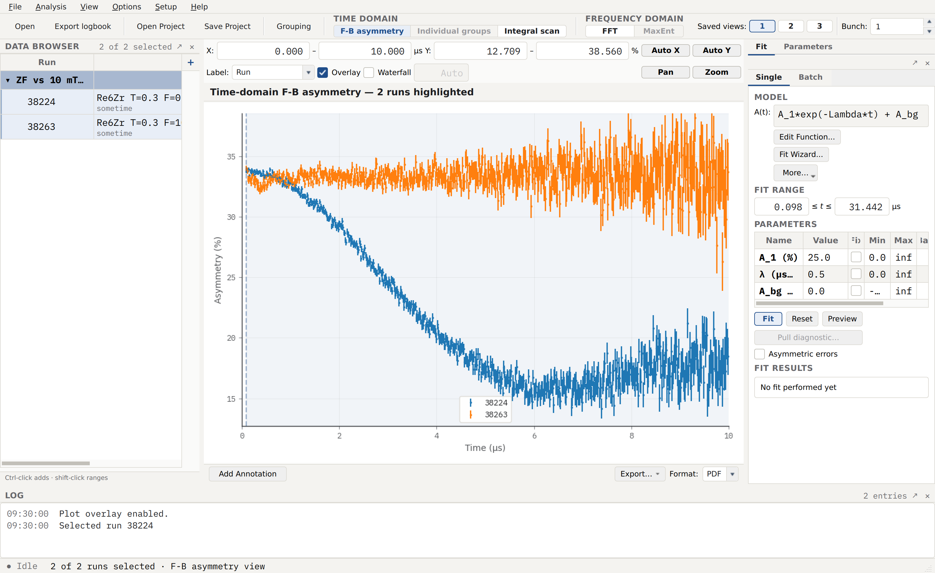
Re₆Zr base-temperature zero-field spectrum overlaid with the 10 mT longitudinal-field spectrum — The static case, for contrast: the superconductor Re₆Zr at base temperature (0.3 K), zero field (blue, 38224) overlaid with 10 mT longitudinal field (orange, 38263). The zero-field trace relaxes toward its Kubo–Toyabe 1/3 tail; a mere 10 mT (100 G) of longitudinal field flattens it completely. This is the discriminating diagnostic — a single small field fully decouples a static distribution.

The Ca₃Co₂O₆ plateau is dynamic; Re₆Zr’s spontaneous fields below its superconducting \(T_c\) are static, and the same LF geometry proves it the opposite way. In Re₆Zr the relaxation is a Gaussian Kubo–Toyabe with a width \(\Delta \approx 0.26\;\mu\mathrm{s}^{-1}\) — equivalent to an internal field of only a few gauss — so a longitudinal field of 10 mT is a hundredfold larger than the internal width and decouples the muon completely. The relaxation switches off at a fixed, small field, and does not fall smoothly with increasing field as a dynamic rate would.

That is the whole discriminator in one pair of numbers. A static distribution decouples at a threshold field set by its width and stays decoupled; a dynamic distribution keeps relaxing to far higher fields, with a rate that falls as \(1/B^2\). Ca₃Co₂O₆ still shows a measurable \(\lambda = 0.3\;\mu \mathrm{s}^{-1}\) at 3.8 T; Re₆Zr is flat by 10 mT. The two corpus datasets bracket the diagnostic — dynamic Redfield falloff on one side, a clean static decoupling threshold on the other. The Re₆Zr measurement is worked in full, including the time-reversal-symmetry-breaking signature it was designed to find, in the superconductivity chapters.

The static LF-KT decoupling series

Neither corpus dataset shows a full static decoupling series — Ca₃Co₂O₆ is dynamic, and the Re₆Zr contrast uses only two fields. The textbook static case, where the LF-KT polarisation is measured across a progression of fields spanning \(\gamma_\mu B_L/\Delta \in \{0, 1, 2, 5, 10\}\), is best shown on a synthetic silver dataset, for which the answer is known exactly.

Converged global LF-KT fit on a synthetic Ag decoupling series

The model for every run is LongitudinalFieldKT + Constant, fitted jointly across the field series in a global fit: the Gaussian width \(\Delta\) is shared (Global), the applied field \(B_L\) is fixed per run (File), and the initial asymmetry and background are shared. Hayano et al. computed the full LF-KT polarisation function, which recovers to unity once \(\gamma_\mu B_L \gg \Delta\). For the synthetic Ag series with input \(\Delta = 0.39\;\mu\mathrm{s}^{-1}\) the global fit recovers \(\Delta = 0.3902\;\mu\mathrm{s}^{-1}\) with per-run reduced \(\chi^2\) near unity, and the diagnostic is read off the highest-field run: because it flattens to \(A_0 + A_{bg}\) within the fit uncertainty, the distribution is confirmed static and \(\Delta\) is the final answer. Were that run still relaxing, the LF-KT model would fail and the dynamic Redfield analysis above would be required instead.

Interpretation

What the analysis delivers:

Static vs dynamic. The shape of \(\lambda(B_L)\) is the diagnostic: a smooth \(1/B^2\) falloff over several tesla is dynamic (Ca₃Co₂O₆); a sharp decoupling at a fixed small field is static (Re₆Zr). This distinction is invisible in a single zero-field spectrum.
Field width \(\Delta\). For the dynamic plateau, \(\Delta = 41.0\;\mathrm{mT}\) is the width of the fluctuating internal field distribution — the spread of local fields the muon samples. For a static case it is instead read from the decoupling threshold or a KT fit.
Correlation time \(\tau\). Only a dynamic scan yields this: \(\tau = 929\;\mathrm{ps}\) is the timescale on which the plateau’s internal fields fluctuate, otherwise inaccessible to a single measurement.
Site and model cross-checks. \(\Delta\) can be compared against a calculated dipolar tensor (via MuFinder or μ-LFC) to confirm the muon stopping site, and the whole scan cross-checks the Redfield model against the independently-known plateau boundaries.

Common pitfalls

Fitting the unresolvable low-field runs. Below ~0.2 T the fast relaxation is beyond the ISIS pulse width and the asymmetry is suppressed, so the single exponential is degenerate and \(\lambda\) collapses to a spurious near- zero minimum. These points are physically meaningless and are excluded from the trend (they appear as ringed markers) — this is a property of the pulsed source, not a program fault.
Forgetting the field-growing background. The constant background rises from ~7 % at 1 T to ~37 % at 3.5 T as decay positrons spiral in the applied field. Fit it (the additive Constant term) rather than assuming a field-independent baseline, or the recovered \(\lambda\) and \(A_1\) are biased.
Reading dynamic where the data are static. A single flat high-field spectrum is consistent with both a decoupled static distribution and a weakly-relaxing dynamic one. Only the field dependence of \(\lambda\) discriminates — always scan several fields before concluding.
Confusing the axis-scale log toggle with a transform. The Redfield linearisation needs the plotted values transformed (reciprocal Y, square X), not merely the tick spacing changed. The log checkbox rescales the ticks and leaves the numbers alone; use the Axis transforms section for the linearisation (Parameter trending).

Cross-references

Parameter trending — the trending panel, axis transforms, and the trend model-fit dialog used for the Redfield linearisation.
Kubo–Toyabe — the static and LF-KT reference page.
Muon diffusion in copper: Kubo–Toyabe, Abragam, and QLCR — the dynamic Kubo–Toyabe worked example (fitting the fluctuation rate \(\nu\) directly).
Global fit wizard — the Global Fit Wizard used for the synthetic LF-KT series.