F–µ–F entangled states: measuring a bond length with muons

Most muon-spin experiments read out a field — the internal field of a magnet, the width of a nuclear-dipolar distribution, the penetration depth of a superconductor. This chapter does something different: it reads out a distance. When a positive muon stops in a fluoropolymer it binds between two fluorine nuclei and the three spins evolve as a single quantum-entangled object, whose zero-field polarisation beats at frequencies fixed entirely by the muon–fluorine separation. Fit that beating and you have measured a sub-ångström bond length with a spin-½ probe — a genuine quantum ruler. The worked example is poly-tetrafluoroethylene (PTFE, Teflon, (–CF₂–CF₂–)_n), the textbook host for the effect, using real MuSR data from the ISIS pulsed source.

This page is a companion to the Nuclear dipolar fit-function reference, which sets out the whole F–µ–F model family and the dipolar Hamiltonian behind it; here the focus is the end-to-end workflow on real data — calibrate, recognise the signature, fit the bond length, and read the frequency-domain view — and, just as importantly, an honest account of where the simplest model stops being adequate.

Why PTFE hosts an entangled three-spin state

PTFE has no double bonds and no unpaired electrons, so the implanted µ⁺ stays diamagnetic — no muoniated radical forms. What it does instead is exploit fluorine’s extreme electronegativity: the muon sits between two F⁻ ions and pulls them towards it into a nearly linear, hydrogen-bond-like F⁻–µ⁺–F⁻ unit. The muon (\(I = 1/2\)) and the two ¹⁹F nuclei (\(I = 1/2\), 100 % abundant, no quadrupole) are coupled by the magnetic dipole–dipole interaction into a closely bound three-spin system. In zero applied field the muon polarisation does not simply relax; it oscillates in a characteristic non-exponential pattern — a deep dip followed by a partial recovery and further beats — that is the unmistakable fingerprint of the coupled centre.

The reason this measures a length is that the whole pattern is governed by one frequency. The zero-field polarisation of the collinear centre beats at three combination frequencies in the ratio \((0.63, 1.73, 2.37)\), all scaled by a single dipolar frequency

\[\nu_d = \frac{\mu_0\,\gamma_\mu\gamma_F\hbar}{16\pi^2\,r_{\mu F}^{3}},\]

which depends on nothing but the muon–fluorine distance \(r_{\mu F}\) (\(\gamma_\mu/2\pi = 135.5\) MHz T⁻¹, \(\gamma_F/2\pi = 40.05\) MHz T⁻¹). Because \(\nu_d \propto r_{\mu F}^{-3}\), fitting the beat frequency returns the bond length directly. That is the deliverable of the classic muon-school exercise on this dataset: fit the F–µ–F relaxation function and derive the dipolar coupling frequency — and hence \(r_{\mu F}\).

The runs

The corpus example ships 30 MuSR runs collected on 22–23 April 2008 on a Teflon sample. One is a transverse-field calibration run; the rest are a zero-field temperature scan.

Run(s)	Field / mode	Role
17293	TF 20 G (cooling)	Calibration run — its transverse precession fixes the detector balance \(\alpha\) before any zero-field analysis.
17294–17322	ZF (0 G)	29 zero-field runs spanning roughly 20–200 K. Run 17294 (20 K, 41.6 MEv) is the highest-statistics base-temperature run and carries the cleanest F–µ–F beating in the set.

Every analysis run is zero-field: the F–µ–F coupling is nuclear and only weakly temperature-dependent, so the physics is essentially the same across the scan, and a single high-statistics base-temperature fit is the robust headline result. The files are ISIS NeXus (HDF4) histograms, which the loader reads natively.

Step 1 — Calibrate α on the transverse-field run

Every time-domain analysis starts from a balanced asymmetry, so the first job is to calibrate \(\alpha\), the forward/backward detector normalisation, on the one transverse-field run in the set. Load run 17293 and view it in the time domain.

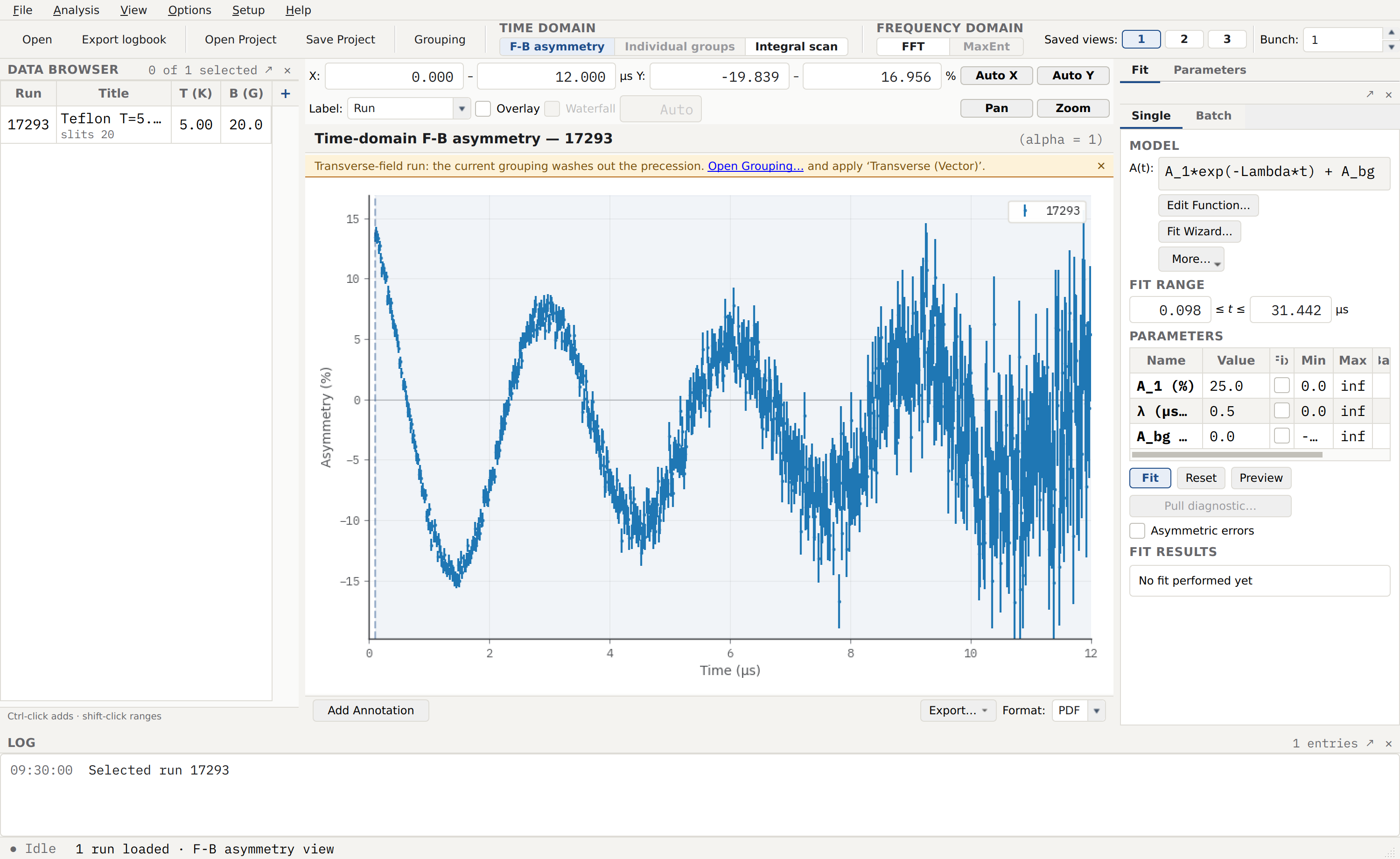
The TF 20 G calibration run 17293 (Teflon, cooling), framed over the first 12 µs. The 20 G field drives a slow transverse precession — \(\gamma_\mu B \approx 0.27\) MHz, a period of about 3.7 µs — and it is the amplitude of this oscillation that fixes the detector balance. The advisory banner (“Transverse-field run: the current grouping washes out the precession. Open Grouping… and apply ‘Transverse (Vector)’.”) points to the Grouping and calibration walkthrough dialog, where Grouping and the α estimate are performed; the plot is still at alpha = 1 (uncalibrated) here. Past about 8 µs the forward and backward counts have run down and the raw asymmetry ratio grows noisy, which is normal for pulsed MuSR data and does not affect the estimate.

With \(\alpha\) calibrated, every zero-field run in the scan inherits the same detector balance.

Step 2 — Read the raw zero-field signature

Before fitting anything, load the base-temperature zero-field run and look at the raw asymmetry. The F–µ–F signature is distinctive enough to identify by eye, and recognising it is half the analysis.

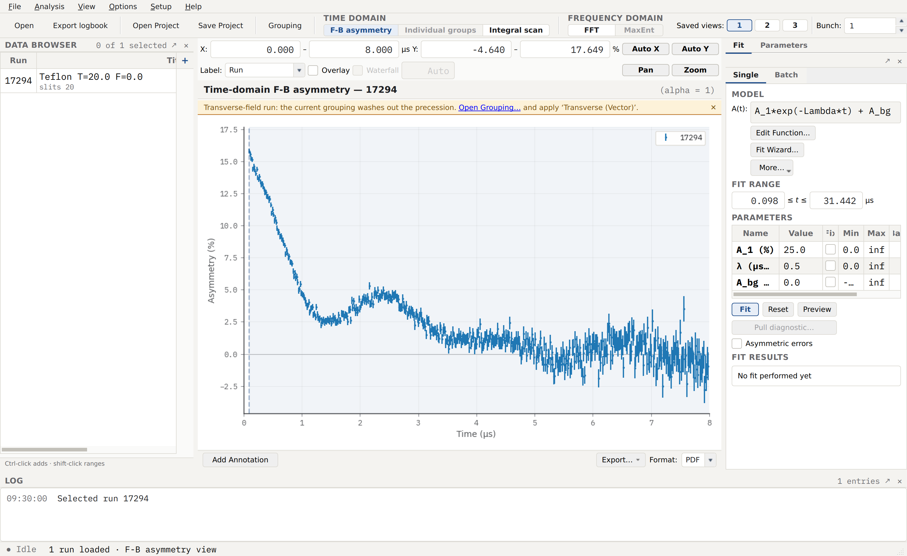
The raw zero-field asymmetry of run 17294 (20 K), framed over the first 8 µs. This is the F–µ–F fingerprint: the polarisation falls from its ~15 % initial value into a deep dip near 1.3 µs, recovers into a bump near 2.2 µs, and beats once more before decaying into the baseline by about 4 µs. A simple relaxation — exponential or Gaussian — cannot produce the recovery; only a coherent, oscillating few-spin polarisation can. The non-monotonic dip-and-recovery is the direct time-domain evidence that the muon has formed a coupled F–µ–F centre, and its period sets the dipolar frequency the fit will quantify.

Step 3 — Fit the F–µ–F polarisation and read off the bond length

The dedicated model is FmuF_Linear — the analytic zero-field polarisation of the collinear three-spin centre, parameterised directly by \(r_{\mu F}\) in ångström (see FmuF_Linear). Fitting it alone, however, fails: the oscillation in real PTFE damps faster than the bare three-spin form predicts, because each F–µ–F unit also feels weaker couplings to more distant fluorines along the chain. Left uncompensated, the fit drives \(r_{\mu F}\) to its bound. The remedy is to multiply the polarisation by a Gaussian damping envelope, which absorbs those distant-neighbour couplings, and add a flat Constant background. The composite is entered as FmuF_Linear * Gaussian + Constant, which Asymmetry assembles as

A(t): A_1*G_FmuF_linear(t,r_muF) exp(-(sigma*t)^2) + A_bg

The collinear F–µ–F polarisation and the frequency–distance relation

For the symmetric linear centre — muon midway between two equivalent fluorines, the weak F–F coupling neglected — the zero-field polarisation has the closed form

\[G_{F\mu F}(t)=\frac{1}{6}\Big[3 + \cos(\sqrt{3}\,\omega_d t) + \Big(1-\tfrac{1}{\sqrt{3}}\Big) \cos\big(\tfrac{3-\sqrt{3}}{2}\,\omega_d t\big) + \Big(1+\tfrac{1}{\sqrt{3}}\Big) \cos\big(\tfrac{3+\sqrt{3}}{2}\,\omega_d t\big)\Big],\]

an oscillation at the three combination frequencies \(\tfrac{3-\sqrt{3}}{2}\,\omega_d\), \(\sqrt{3}\,\omega_d\), and \(\tfrac{3+\sqrt{3}}{2}\,\omega_d\) — the \((0.63, 1.73, 2.37)\) ratio quoted above. The dipolar coupling \(\omega_d = (\mu_0/4\pi)\,\gamma_\mu\gamma_F\hbar\,r_{\mu F}^{-3}\) carries the whole distance dependence, so the fit reports \(r_{\mu F}\) rather than a frequency. The full model family — including the numerically powder-averaged variants — is documented at Nuclear dipolar.

Seed the amplitude near the ~15 % initial asymmetry, \(r_{\mu F}\) at the literature guidance value of about 1.15 Å, and the Gaussian width near 0.35 µs⁻¹, then press Fit.

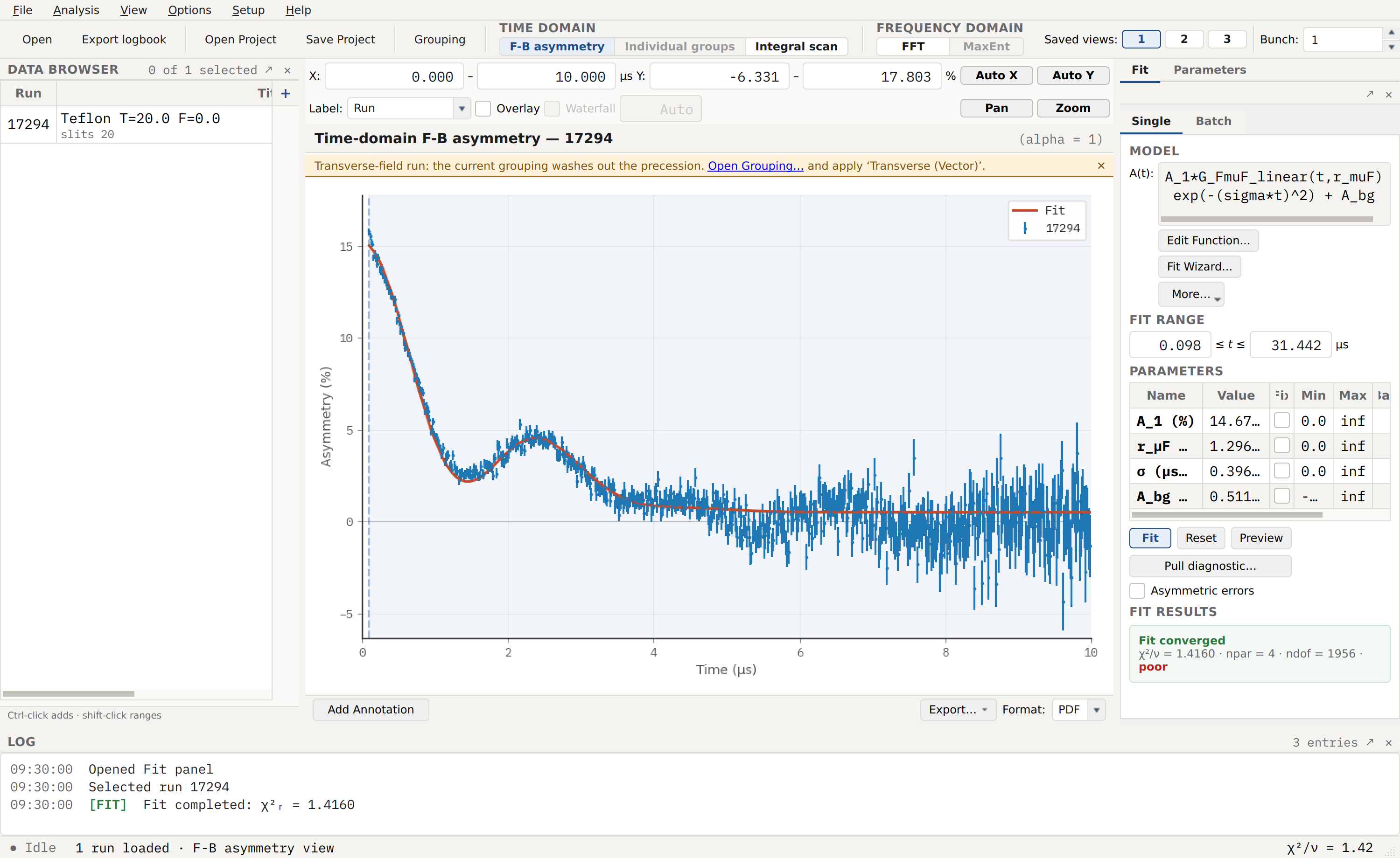
The converged FmuF_Linear * Gaussian + Constant fit on run 17294, framed over the first 10 µs where the beats and the fit overlay both read. The red Fit curve traces the dip and recovery cleanly. The Parameters table reports the fitted amplitude \(A_1 = 14.68(5)\) %, the muon–fluorine distance \(r_{\mu F} = 1.296(1)\) Å, the Gaussian damping \(\sigma = 0.396(3)\) µs⁻¹, and a small residual background \(A_{bg} = 0.51(3)\) %. The Fit results chip reads Fit converged, χ²/ν = 1.4160 · npar = 4 · ndof = 1956, with a quality verdict of poor — a point taken up below.

The headline number is \(r_{\mu F} = 1.30\) Å — a bond length measured to about a picometre from a spin oscillation. It is the right order of magnitude and carries the correct physics, but it sits above the literature band of 1.1–1.2 Å (Brewer et al. found 1.172 Å in CaF₂), and the quality chip flags the fit as poor. Both facts are honest and instructive rather than embarrassing — see the next section.

Note

This corpus dataset is an unallocated 2008 teaching run, not the data behind any publication, and the muon-school guide sets no numeric target for the bond length or the frequency. The 1.1–1.2 Å figure is a literature expectation for the same physics (an ionic-fluoride and fluoropolymer value), used here only as a sanity check on a physically sensible result.

Step 4 — The frequency-domain view

The same beating can be read as a spectrum. Switch to the FFT view; the three combination lines of the F–µ–F centre sit sub-MHz, on the skirt of the large zero-frequency (DC) term left by the decaying envelope. Because that DC skirt dominates the raw transform, an apodisation filter matched to the beat’s coherence time is what makes the F–µ–F structure legible.

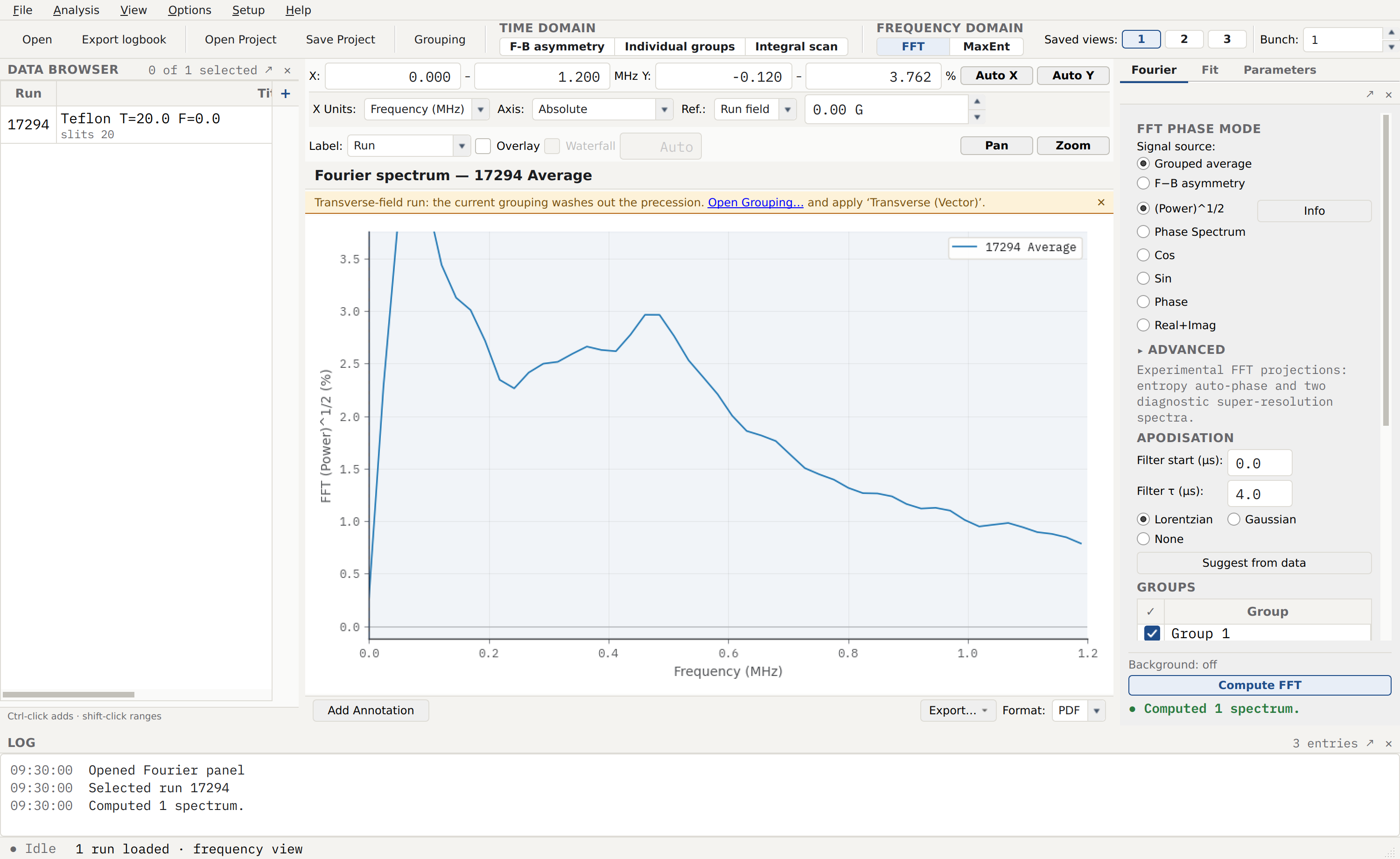
The Fourier spectrum of run 17294 over 0–1.2 MHz. The broad sub-MHz F–µ–F line cluster peaks near 0.47 MHz — the frequency-domain image of the time-domain beating — riding on the DC skirt, which is framed to run off the top so the cluster stays legible. The Fourier inspector on the right carries the transform’s own controls: the Apodisation section is set to a Lorentzian filter with Filter τ (µs) of 4.0, matched to the beat’s coherence time to trim the noisy record tail, with Suggest from data available to choose it automatically; the signal source is Grouped average displayed as (Power)^1/2. The line cluster is broad under an ordinary FFT — sharpening it into the three resolved combination lines is the natural application of the MaxEnt estimator (Fourier analysis).

Assumptions and limitations

• The fitted distance is biased high, and this is a model limitation. FmuF_Linear assumes a perfectly collinear, symmetric centre with two equivalent fluorines at a single distance \(r_{\mu F}\). In PTFE the local geometry is neither exactly linear nor exactly symmetric, and forcing the collinear form onto a slightly bent unit — together with the Gaussian envelope absorbing part of the early-time curvature — pushes the fitted \(r_{\mu F}\) upward, to ~1.30 Å against the 1.1–1.2 Å expectation. The refinement route is to relax the geometry: FmuF_General fits two inequivalent distances and a bond angle (\(r_1, r_2, \theta\)), and FmuF_Triangle adds a third fluorine. Both are numerically powder-averaged and considerably slower than the analytic collinear form, so the collinear fit is the right first model and the excess distance is the signal to try the more general ones (see FmuF_General and FmuF_Triangle).

• A “poor” χ² verdict is itself a teaching point. The reduced \(\chi^2_\nu = 1.42\) is flagged poor not because the fit is wrong but because, over ~1956 degrees of freedom, the systematic mismatch between a collinear model and a bent centre is statistically resolvable. The chip is reporting a real inadequacy of the model, and reading it that way — rather than tuning seeds to chase a smaller number — is the correct response.

• The damping envelope is a modelling choice, not a prescribed term. The guide names only “the FmuF relaxation function”; the Gaussian envelope is added because the bare centre over-oscillates. A Lorentzian (Exponential) envelope is the alternative used for cleaner F–µ–F powders, and the choice shifts the fitted \(r_{\mu F}\) slightly. Neither the envelope nor the fit window is fixed by the physics.

• One temperature, by design. The F–µ–F coupling is nuclear and only weakly temperature-dependent, so a bond-length-versus-temperature trend would be nearly flat; the single high-statistics base-temperature fit is the robust deliverable. Fits at higher temperatures need warm-starting from the base-temperature result — from fixed guidance seeds alone, a warmer run can walk \(r_{\mu F}\) into a bad local minimum at its bound. If instead the oscillation visibly washes out on warming because the muon begins to hop, DynamicFmuF (DynamicFmuF) is the model that turns that damping into a hop rate.

References

• J. H. Brewer, S. R. Kreitzman, D. R. Noakes, E. J. Ansaldo, D. R. Harshman, and R. Keitel, Phys. Rev. B 33, 7813 (1986) — the discovery of the F–µ–F “hydrogen-bonded” centre in ionic fluorides, and the collinear three-spin polarisation function used here (\(r_{\mu F} = 1.172\) Å in CaF₂).

• T. Lancaster, F. L. Pratt, S. J. Blundell, I. McKenzie, and H. E. Assender, J. Phys.: Condens. Matter 21, 346004 (2009) — muon–fluorine entanglement in fluoropolymers, the modern treatment of the F–µ–F state in PTFE and related materials.

• F. L. Pratt, S. J. Blundell, I. M. Marshall, T. Lancaster, A. Husmann, C. Steer, W. Hayes, C. Fischmeister, R. E. Martin, and A. B. Holmes, Physica B 326, 34 (2003) — µSR in polymers.

• K. Nishiyama, S. W. Nishiyama, and W. Higemoto, Physica B 326, 41 (2003) — the asymmetric F–µ–F interaction in polyfluorocarbons.

• S. J. Blundell, R. De Renzi, T. Lancaster, and F. L. Pratt, Muon Spectroscopy: An Introduction (Oxford University Press, Oxford, 2022) — nuclear dipolar coupling and F–µ–F states.

Cross-references

• Nuclear dipolar — the full F–µ–F fit-function family: MuF, FmuF_Linear, FmuF_General, FmuF_Triangle, and DynamicFmuF, with the dipolar Hamiltonian behind them.

• Grouping and calibration walkthrough — the grouping profile and α calibration used in Step 1.

• Fourier analysis — the FFT and MaxEnt frequency-domain views and the apodisation controls of Step 4.

• Composite models — building composite models such as FmuF_Linear * Gaussian + Constant.

• Fit wizard — the Fit Wizard, which recognises muon-fluorine bonding and proposes an F–µ–F composite automatically.