Global fitting across fields: Li⁺ ionic motion in a garnet electrolyte

This chapter is the flagship worked example of a global fit — a single simultaneous fit of several runs that share some parameters and differ in others. It takes a real longitudinal-field (LF) decoupling series measured on EMU at ISIS and, one temperature at a time, fits a triplet of runs recorded at three applied fields with one shared model, then trends the fitted fluctuation rate against temperature to recover an activation energy for lithium-ion motion. The sample is an aluminium-doped lithium garnet, Li₇La₃Zr₂O₁₂ (LLZ), a candidate solid electrolyte for a lithium-ion battery; the same runs were published by Amores et al., J. Mater. Chem. A 4, 1729 (2016), so the analysis here has a paper-grade target to aim at.

Its synthetic sibling, LF decoupling and static-vs-dynamic field distributions, builds the same story on a textbook Ag decoupling series and works through the static-versus-dynamic formalism in detail. Read that page for the theory of Kubo–Toyabe decoupling; this page is the real-data counterpart and concentrates on why you need a global fit at all, and on the practical mechanics of tying parameters across a field triplet.

Why a global fit is unavoidable here

In a solid electrolyte the muon spin relaxes because it sits in a fluctuating local field: the nuclear moments of the lithium (and other) ions that diffuse past it produce a field distribution of width \(\Delta\) that fluctuates at a rate \(\nu\) set by the ionic hop rate. Both quantities are physical unknowns we want per temperature. The trouble is that a single relaxing curve constrains them only jointly — a broad, slowly-fluctuating distribution and a narrower, faster one can produce almost the same early-time decay. Fitting one field in isolation is therefore degenerate: \(\Delta\) and \(\nu\) trade off against each other along a valley in parameter space, and the fit reports a tightly-correlated pair rather than two independent numbers.

Applying a longitudinal field breaks the degeneracy. A field along the initial muon spin direction progressively decouples the muon from the nuclear fields: as \(\gamma_\mu B_L\) grows the relaxation slows, and how fast it slows with field depends on \(\Delta\) and \(\nu\) in different ways. A run at 0 G, one at 5 G, and one at 10 G thus carry complementary information, and a single model fitted to all three at once — with \(\Delta\) and \(\nu\) forced to take one shared value across the triplet while the field \(B_L\) is held at each run’s own set value — pins both parameters. That simultaneous, parameter-sharing fit is what Asymmetry (and the WiMDA “Multi Fit” it descends from) calls a global fit.

The runs

The corpus example ships 40 EMU runs collected in April 2015 (experiment RB1510349): one transverse-field calibration run and thirteen temperatures each measured at three longitudinal fields.

Run(s)	Field / mode	Role
51315	TF 20 G (300 K)	Calibration run — its precession amplitude fixes the detector balance \(\alpha\) before any science fit.
51341–51379	LF 0 / 5 / 10 G	13 temperatures × 3 fields = 39 science runs. Each temperature’s triplet is the three consecutive runs (zf, zf+1, zf+2) = (0 G, 5 G, 10 G); the zero-field run opens each set (51341, 51344, … 51377).

The temperature setpoints span 160–404 K (measured sample temperatures 157–391 K). All 40 files are HDF4-based ISIS NeXus histograms; the EMU loader reads each run’s applied field and setpoint temperature straight from the file header, which — as the workflow below relies on — means the per-run field can be supplied to the fit automatically rather than typed in by hand.

Step 1 — Calibrate α from the TF run

Every time-domain analysis starts from a balanced asymmetry, so the first job is to calibrate \(\alpha\), the forward/backward detector normalisation, on the transverse-field run 51315. The full mechanics of the grouping profile and the calibration dialog are covered in EMU detector grouping and α calibration; here it is a single preparatory step.

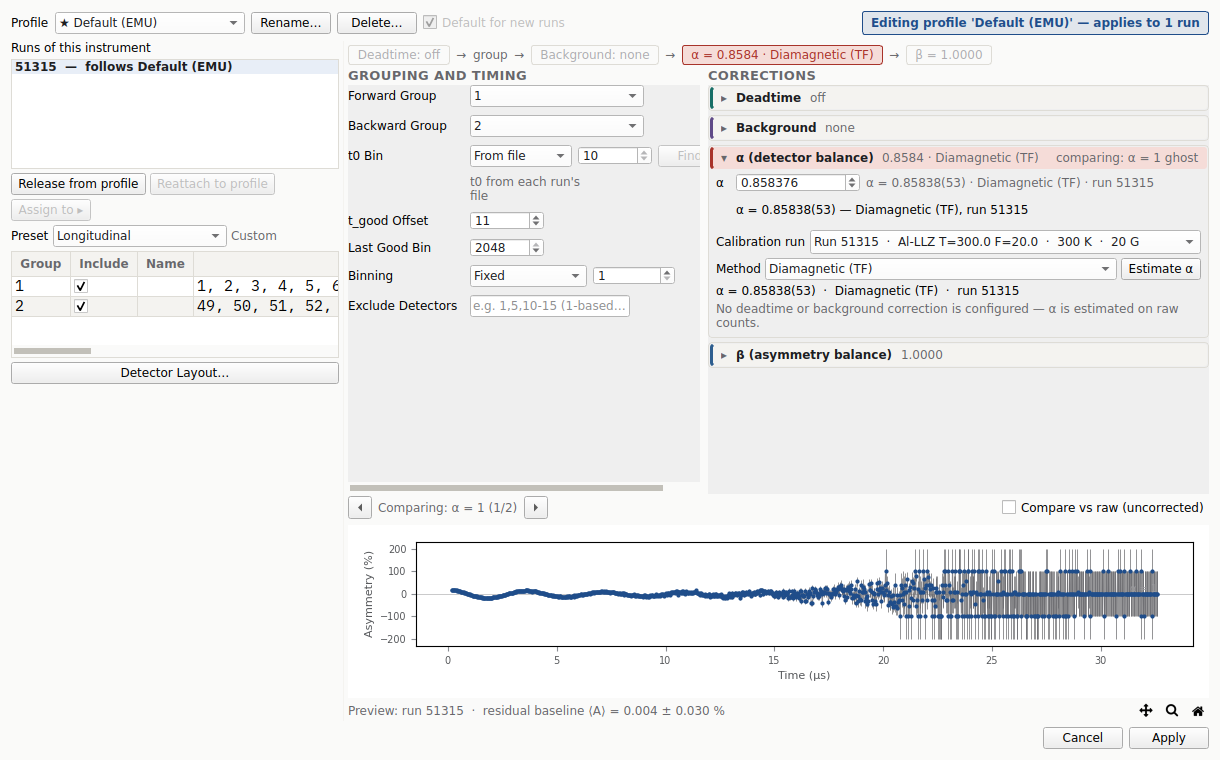
The inline alpha calibration (the Grouping window’s α (detector balance) card) on the TF 20 G run 51315. With the Diamagnetic (TF) method selected, Estimate α finds the \(\alpha\) that makes the transverse-field precession oscillate symmetrically about zero; the α card reports \(\alpha = 0.876\) for this silver-free garnet run. The grey \(\alpha = 1\) (before) and blue fitted (after) traces show the balancing directly. The precession is clean out to about 20 µs; past ~25 µs the forward/backward counts have run down and the raw asymmetry ratio grows noisy, which is normal for pulsed EMU data and does not affect the estimate.

With \(\alpha\) calibrated and the grouping profile applied, every LF run of the series inherits the same detector balance automatically.

Step 2 — Read the raw field triplet

Before fitting anything, load one temperature’s triplet and overlay the three fields. This is where the decoupling signature — and the case for a joint fit — becomes visible.

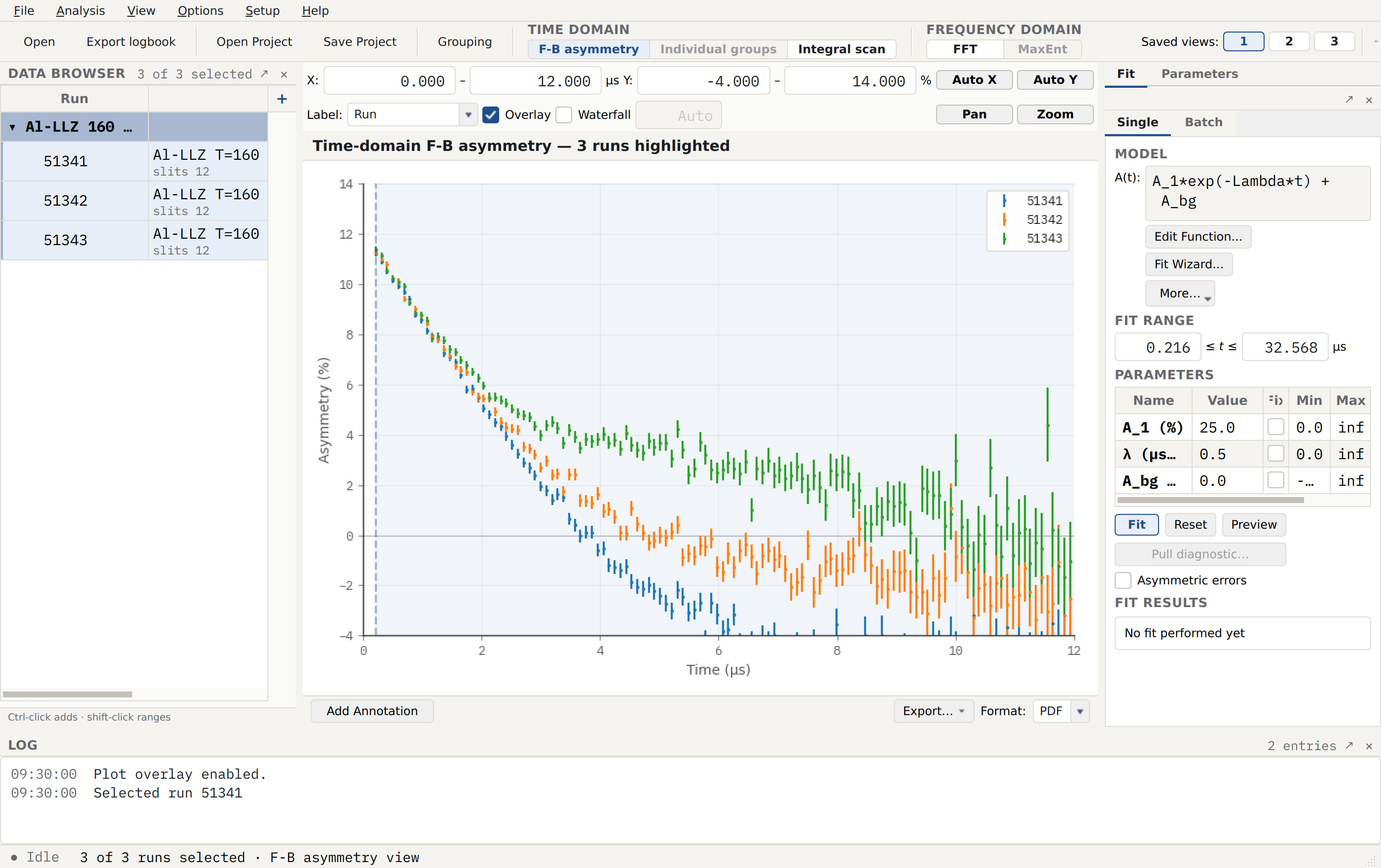
The 160 K triplet — runs 51341 (0 G), 51342 (5 G) and 51343 (10 G) — loaded into a data group and drawn with Overlay enabled. The three fields separate clearly: the zero-field trace (blue) relaxes fastest, the 5 G trace (orange) more slowly, and the 10 G trace (green) least of all. That progressive slowing with field is the decoupling, and each field samples the \((\Delta, \nu)\) pair differently — the raw justification for fitting them together. The plot is clipped to the 0–12 µs analysis window (see the fit-range note below).

The separation between the three curves is modest — this is weak decoupling, only a few gauss — which is exactly why one field alone cannot resolve \(\Delta\) from \(\nu\) and why the three must be fitted jointly.

Step 3 — The model and the parameter classification

The model applied to every run in the triplet is the Keren relaxation function plus a flat background, entered as the composite Keren + Constant. Asymmetry displays its assembled form as

A(t): A_1*exp(-Gamma(t; Delta=Delta, nu=nu, B_L=B_L)) + A_bg

The Keren function is the standard analytic model for LF decoupling by a fluctuating nuclear-dipolar field: it carries the static field-distribution width \(\Delta\), the fluctuation rate \(\nu\), and the applied field \(B_L\) directly as parameters, and is accurate in the fast/intermediate regime that ionic motion occupies. It is the same model Amores et al. used on this dataset. The flat Constant term is the background the guide asks for — muons that stop outside the sample and do not relax.

The Keren relaxation function

Keren’s analytic generalisation of the Abragam function to a longitudinal field gives the muon polarisation as \(A(t) = A\,e^{-\Gamma(t)}\) with

\[\Gamma(t)=\frac{2\Delta^2}{(\omega_0^2+\nu^2)^2} \Big[(\omega_0^2+\nu^2)\,\nu t +(\omega_0^2-\nu^2)(1-e^{-\nu t}\cos\omega_0 t) -2\nu\omega_0\, e^{-\nu t}\sin\omega_0 t\Big],\]

where \(\omega_0 = \gamma_\mu B_L\) is the muon Larmor frequency in the applied longitudinal field. It is a strong-collision result valid when \(\nu \gtrsim \Delta\) and reduces to the Abragam function at \(B_L = 0\). The full derivation and parameter list are on the Keren reference page; where fluctuations are slow (\(\nu \lesssim \Delta\)) the full dynamic Kubo–Toyabe of LF decoupling and static-vs-dynamic field distributions is the better model.

The heart of a global fit is deciding, parameter by parameter, whether a quantity is shared across the runs or individual to each. That decision is made in the Batch tab’s Parameter classification table.

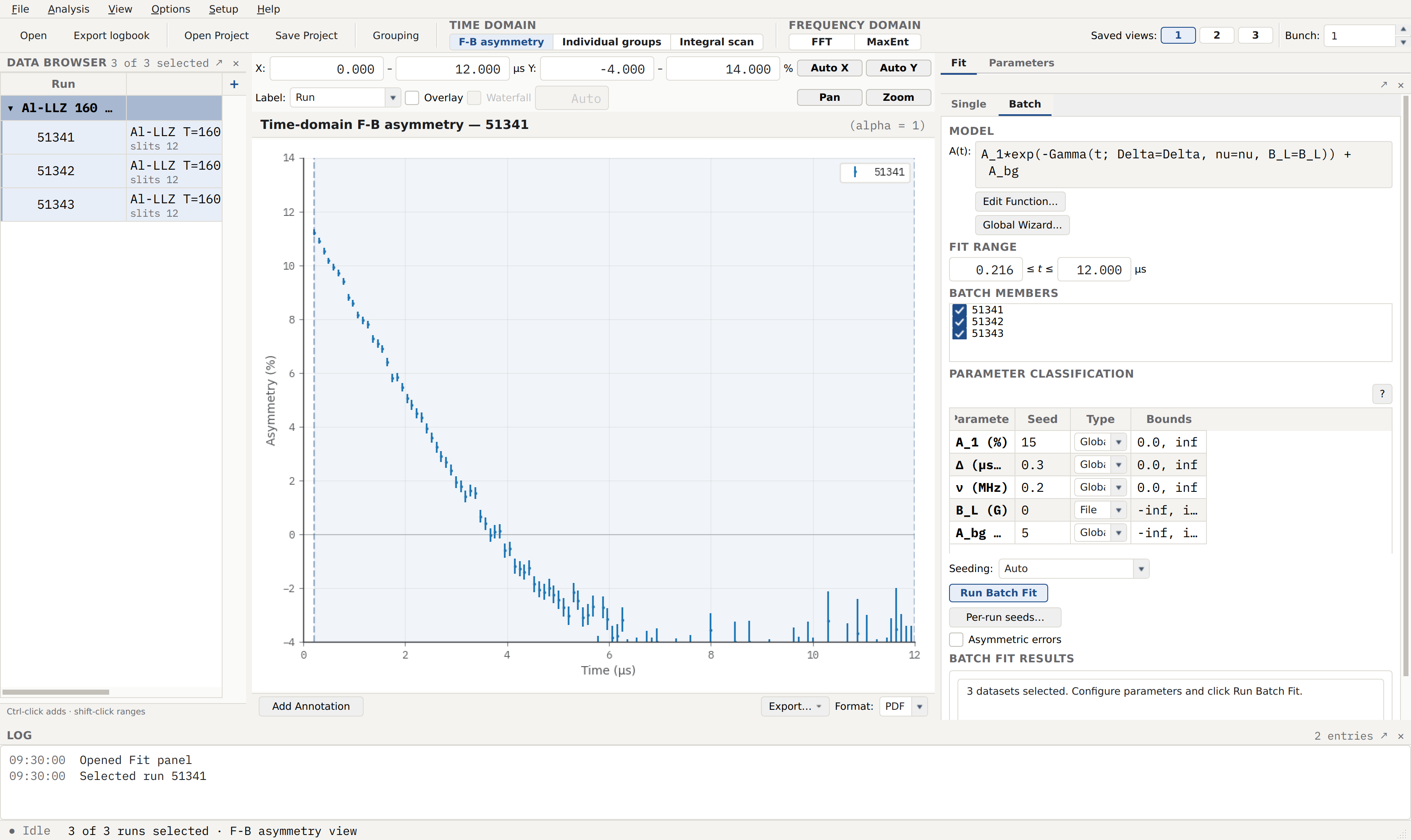
The Batch tab set up for the joint fit of the 160 K triplet. The Parameter classification table is the whole story of the fit: each row’s Type decides whether that parameter is shared or per-run. The Fit range is capped at 12 µs and the guide’s seed values are entered in the Seed column, with all three runs selected so Run Batch Fit acts on the loaded triplet.

Walk down the classification table row by row — this is the tying picture that makes the fit a global one:

Parameter	Seed	Type	Role in the joint fit
A_1 (%)	15	Global	Sample-signal amplitude. The relaxing garnet signal is the same physical fraction of the asymmetry at every field, so one shared value serves the triplet.
\(\Delta\) (µs⁻¹)	0.3	Global	Static field-distribution width. This is a property of the sample at this temperature, not of the applied field — one value, shared. Sharing it across fields is precisely what lifts the \(\Delta\)–\(\nu\) degeneracy.
\(\nu\) (MHz)	0.2	Global	Fluctuation (hop) rate — the quantity whose temperature dependence gives the activation energy. Also a sample property, hence shared.
B_L (G)	0	File	Applied longitudinal field. This is the one parameter that differs between the runs, and it is not fitted at all: File fixes it per run to the 0 / 5 / 10 G value read from each run’s own header. This is why the loader reading the field from the file matters.
A_bg (%)	5	Global	Flat background amplitude. Muons stopping outside the sample give the same field-independent background at each field, so it too is shared.

The Type column is the general mechanism: a Global parameter takes one value across every run in the batch; a File parameter is fixed per run to the value stored in that run’s metadata; and a per-run free parameter (Local in the general case) would take an independent fitted value per run. Here only \(B_L\) varies, and it varies in a known way, so the triplet is described by just four shared numbers plus three fixed fields — the textbook shape of a well-posed global fit.

Two practical settings complete the setup. The Fit range is limited to \(t \le 12\) µs: past about 13 µs the forward/backward counts of pulsed EMU data have run down and the asymmetry ratio diverges, so restricting the window both speeds the fit and keeps the noisy tail out of it. The Seed values (\(A_1 = 15\) %, \(A_{bg} = 5\) %, \(\Delta = 0.3\), \(\nu = 0.2\)) are the guide’s suggested starting points at 160 K — starting values, not results. Warm-starting each higher temperature from the previous fit’s converged values (“propagate up in temperature”) makes the whole series converge cleanly.

Step 4 — Run the joint fit

With the triplet selected and the parameters classified, Run Batch Fit performs the simultaneous fit.

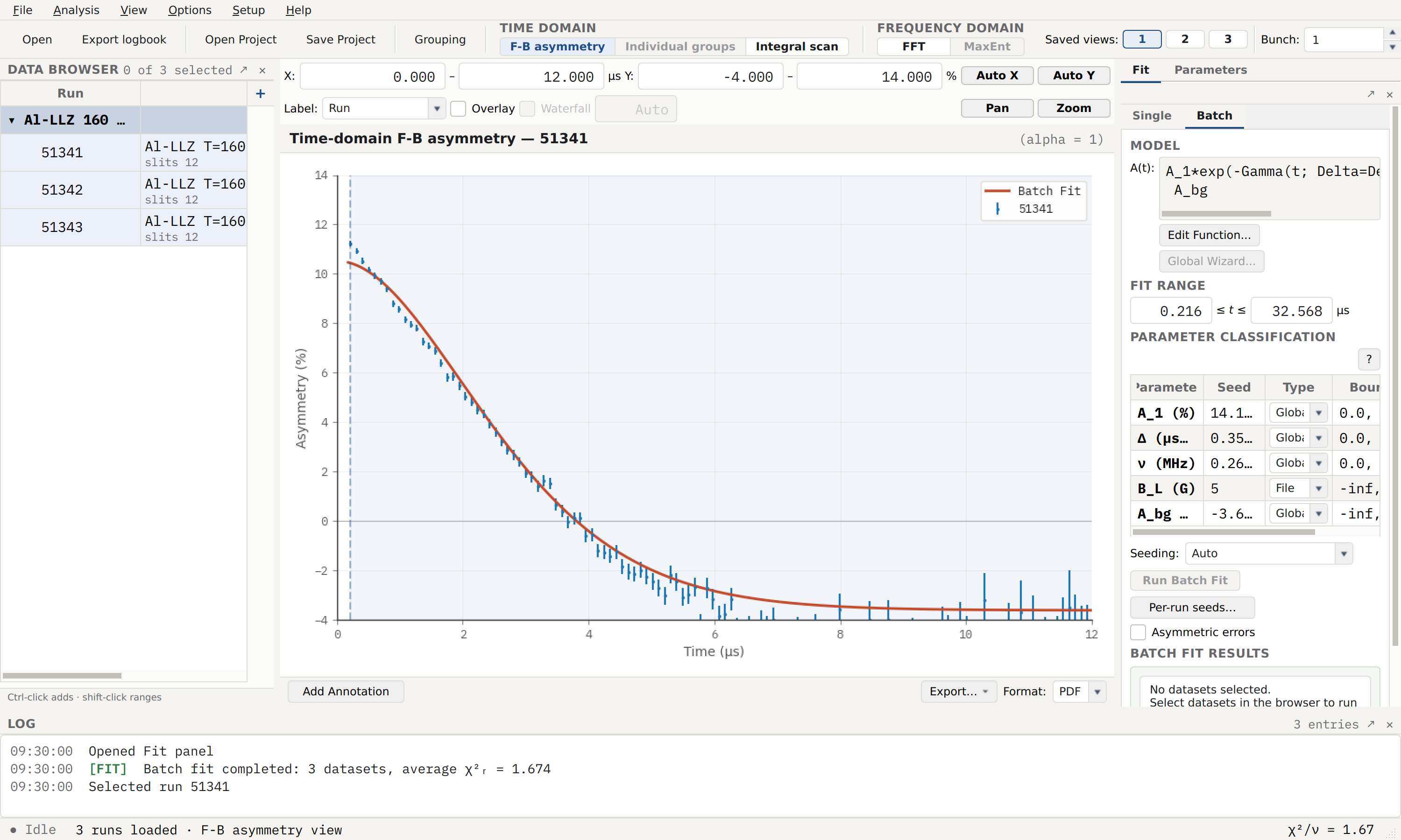
The converged joint fit. The red Batch Fit curve traces the zero-field run cleanly through the decoupling shoulder, and the classification table now carries the fitted shared values: \(\Delta = 0.358\) µs⁻¹ and \(\nu = 0.267\) MHz at 160 K, with \(A_1 = 14.1\) %. The log reports the joint quality, average χ²ᵣ = 1.674 across the three runs — one fit describing all three fields at once.

The fitted \(\Delta = 0.358\) µs⁻¹ and \(\nu = 0.267\) MHz sit close to the guide’s seeds, as expected for the lowest temperature where the ions are nearly frozen. Note that the background amplitude fits to a small negative value here (\(A_{bg} \approx -3.6\) %) rather than the +5 % seed: with a single flat term standing in for the true baseline the fit is free to place it below zero, a reminder that the background model is a modelling choice (see Assumptions and limitations).

Step 5 — Trend ν(T) and extract the activation energy

Repeating the joint fit at all thirteen temperatures builds a \(\nu(T)\) series — the payoff of the whole workflow. Physically we expect \(\nu\) to sit on a low, roughly constant plateau while the lithium ions are immobile and then rise steeply once thermally-activated hopping switches on. In this reproduction \(\nu\) is flat near 0.27 MHz up to about 250 K and then climbs to roughly 1.1 MHz at the top of the range, matching the paper’s “plateau, then activated rise above ~290 K”. (Over the same series \(\Delta\) decreases smoothly — the width the muon sees narrows as the ions mobilise — from 0.358 µs⁻¹ down to about 0.27 µs⁻¹.)

An activation energy comes from an Arrhenius analysis of the rising branch. In the parameter-trending panel this is done natively by transforming the axes so that an Arrhenius law becomes a straight line, then fitting a Linear model to it.

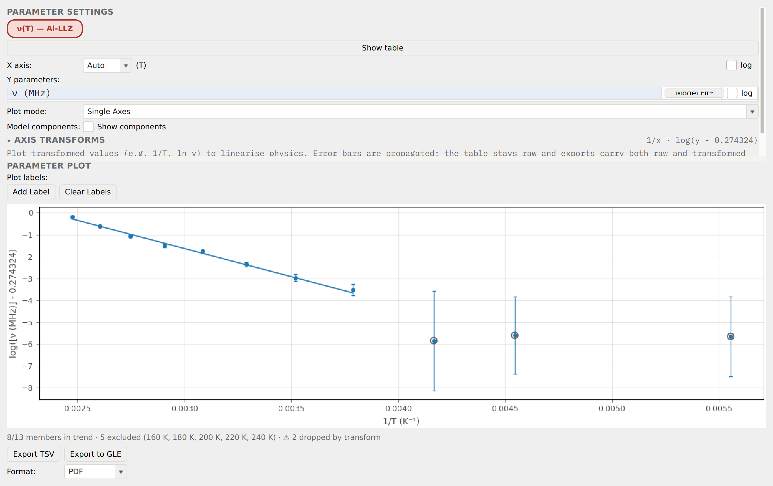
The \(\nu(T)\) trend as a native Arrhenius plot. The abscissa is transformed to \(1/T\) (reciprocal) and the ordinate to \(\log(\nu - 0.274324)\) via a Custom transform; the section chip reads 1/x · log(y - 0.274324). A Linear model fit (Model Fit*) runs on the eight activated-branch points (\(T \ge 264\) K), whose slope is \(-E_a/k_B\). The five plateau points are excluded from the trend (8/13 members in trend · 5 excluded): three sit low with large propagated error bars and two fall below the baseline and drop out entirely.

The reason the transform subtracts a baseline — rather than using the plain \(\ln\) preset — is important, and it is the subtle part of this analysis. The hop rate does not vanish on the low-temperature plateau; it saturates at a residual value \(c \approx 0.274\) MHz. A rate of the form \(\nu(T) = \nu_0\,e^{-E_a/k_BT} + c\) is not linearised by \(\ln\nu\) against \(1/T\), because \(\ln(\nu_0 e^{-E_a/k_BT}+c)\) is not linear in \(1/T\); fitting it returns an activation energy biased low and, worse, one that depends on where the branch is cut. Subtracting the plateau first — the Custom expression log(x - 0.274324) with the plateau value read off the low-temperature end — makes \(\ln(\nu-c)\) genuinely straight and the slope branch-insensitive. The recipe, and the general “Arrhenius on a plateau” caution, are documented under Axis transforms in Parameter trending.

The slope of the fitted line gives

\[E_a = 0.222(8)\ \mathrm{eV},\]

against the paper’s µSR value of \(0.19(1)\) eV from the same data. The two agree in magnitude and both describe the same physics — a lithium-ion hopping barrier of about 0.2 eV, seen locally by the muon. (For contrast, Amores et al. measured 0.55(3) eV by impedance spectroscopy on the same sample; the much larger transport barrier is dominated by inter-grain resistance that the local muon probe does not see — one of the paper’s central points.) The residual ~15 % gap between this reproduction and the paper’s µSR number is honest and attributable: the background model is not uniquely pinned, and there is a known factor-of-\(2\pi\) ambiguity in whether \(\Delta\) and \(\nu\) are quoted in MHz or in angular µs⁻¹.

From the hop rate to a diffusion coefficient

Amores et al. convert the fluctuation rate into a lithium diffusion coefficient with a jump-diffusion (Einstein) relation summed over the two distinct Li hop paths in the garnet structure (24d → 96h and 96h → 24d):

\[D = \sum_i \frac{1}{N_i}\, Z_{v,i}\, s_i^2\, \nu,\]

where for hop path \(i\), \(N_i\) is the number of accessible sites, \(Z_{v,i}\) the destination vacancy fraction, and \(s_i\) the jump distance. Using the measured room-temperature \(\nu\), the paper reports \(D = 4.62\times10^{-11}\ \mathrm{cm^2\,s^{-1}}\) and a mobile Li-ion fraction of 21.7 %. Asymmetry does not compute \(D\) itself — it stops at \(\nu(T)\) and \(E_a\) — but the extracted rate is the input this relation needs.

Assumptions and limitations

• The background model is a choice. The guide asks for “some choice of background terms” without prescribing one; a single flat Constant is the simplest, and it can fit slightly negative (as at 160 K above) when it stands in for a baseline the data do not tightly constrain. A different background (an extra relaxing term, a second Keren component) would shift the fitted \(\Delta\) and \(\nu\) somewhat, and is part of the residual gap to the paper’s \(E_a\).

• Δ and ν units carry a 2π ambiguity. Field-distribution widths and hop rates in Keren/dynamic-KT parameterisations are variously quoted in MHz or in angular µs⁻¹, which differ by \(2\pi\). The seeds are taken as the guide’s literal values; do not assume a conversion when comparing numbers across sources.

• The Keren caveat at low temperature. The Keren function is a fast-fluctuation result and “does not work for both zero field and low fluctuation rate”, so at the lowest temperatures the zero-field run can be excluded, fitting only the 5 / 10 G pair. Here all three fields are kept — the joint fits converge with \(\chi^2_r \le 1.7\) at every temperature — but on data where the ZF run pulls the low-temperature fit, dropping it (or switching to the full dynamic Kubo–Toyabe, which the guide names as the alternative model) is the correct response.

• The Arrhenius branch and baseline are chosen by eye. The activated branch (\(T \ge 264\) K) and the plateau baseline (\(c = 0.274\) MHz) are read off the trend, not fitted jointly; the extracted \(E_a\) is reassuringly insensitive to exactly where the branch is cut once the baseline is subtracted, but a different baseline would move it. The alternative is to skip the linearisation and fit an Arrhenius model in raw coordinates.

• Setpoint versus measured temperature. The trend axis uses the nominal setpoints (160–404 K); the instrument-recorded sample temperatures run systematically lower (157–391 K). For a higher-precision Arrhenius slope, trend against the logged temperatures instead (see How the T / B abscissa is sourced).

References

• M. Amores, T. E. Ashton, P. J. Baker, E. J. Cussen, and S. A. Corr, J. Mater. Chem. A 4, 1729 (2016) — the published analysis of this dataset: EMU LF 0/5/10 G decoupling, a simultaneous Keren fit at each temperature, and the Li⁺ activation energy \(E_a = 0.19(1)\) eV.

• A. Keren, Phys. Rev. B 50, 10039 (1994) — the analytic longitudinal-field relaxation function used here.

• R. S. Hayano, Y. J. Uemura, J. Imazato, N. Nishida, T. Yamazaki, and R. Kubo, Phys. Rev. B 20, 850 (1979) — the dynamic Kubo–Toyabe theory of field decoupling that Keren’s function generalises.

• S. J. Blundell, R. De Renzi, T. Lancaster, and F. L. Pratt, Muon Spectroscopy: An Introduction (Oxford University Press, Oxford, 2022), Ch. 5 — LF decoupling and dynamic relaxation.

Cross-references

• LF decoupling and static-vs-dynamic field distributions — the synthetic sibling: the static-versus- dynamic Kubo–Toyabe formalism behind LF decoupling, worked on a textbook Ag series.

• EMU detector grouping and α calibration — the EMU grouping profile and α calibration used in Step 1.

• Keren — the Keren fit-function reference page.

• Global fit wizard — the Global Fit Wizard for automated role selection.

• Parameter trending — the trending panel, axis transforms, and the Arrhenius-on-a-plateau recipe.

• Composite models — building composite models such as Keren + Constant.