Photo-μSR in silicon: carrier recombination from period-mode runs

Photoexcited muon-spin spectroscopy turns the muon into a contactless probe of excess charge carriers in a semiconductor. A pulsed laser injects electron–hole pairs into intrinsic silicon; the implanted μ⁺ captures an electron to form muonium (Mu = μ⁺ + e⁻), and the excess carriers relax the muon spin through the hyperfine interaction. The relaxation rate \(\lambda\) therefore acts as a yardstick for the excess carrier density \(\Delta n\), and following \(\lambda\) as the carriers recombine measures the carrier lifetime. This chapter works that analysis end to end on real HiFi data, and doubles as the corpus’s showcase for period-mode files — a single run that holds two histogram sets, laser ON and laser OFF.

The dataset is not a teaching mock-up: runs HIFI00103277–103299 (ISIS proposal RB1520457, May 2016) are the very measurements published in K. Yokoyama et al., Phys. Rev. Lett. 119, 226601 (2017). That makes the example paper-graded — the numbers Asymmetry recovers below can be held against the published fit values, and they agree.

The data

The example uses 23 two-period HiFi (ISIS pulsed source) runs on single-crystal intrinsic silicon (\(R > 1000\;\Omega\,\mathrm{cm}\)) at room temperature (\(T = 291\;\mathrm{K}\)) in a longitudinal field of 100 G (10 mT). They fall into three roles (corpus Semiconductors → Photo-μSR in silicon, Data/):

Calibration set — runs 103277–103286, laser timing \(\Delta T = 0\), injected carrier density stepped from \(\Delta n = 8.9 \times 10^{13}\) down to \(9.3 \times 10^{12}\;\mathrm{cm^{-3}}\). These fix the \(\lambda\)–\(\Delta n\) calibration.
Delay scan — runs 103287–103298, fixed injected density, laser delay \(\Delta T\) stepped from 0.1 to 70 μs. As the delay grows the carriers recombine before the muons probe them, so \(\lambda\) falls; the decay gives the lifetime.
α calibration — run 103299, a transverse-field run at 20 G used to balance the detectors (see EMU detector grouping and α calibration).

The laser fires at 25 Hz against the pseudo-50 Hz muon pulse, so the sample is illuminated on every other pulse. The data-acquisition electronics sort the two cases into two periods within one .nxs file: the muon pulses that arrived with the laser on, and those that arrived with it off. Resolving that structure is the first job of the analysis.

Period-mode data handling: red and green

Load a run and open the Grouping dialog. Period-mode files add an RG Mode row with four choices — Red, Green, G minus R, and G plus R — that select which period (or combination) the reduction uses. The names follow the long-standing WiMDA convention that this experiment reuses: Red = laser ON, Green = laser OFF. Each period carries its own provenance, including its own good-frame normaliser, so dead-time correction and counting statistics stay correct per period.

For runs that carry three or more periods the Map periods… button opens the Map Periods dialog, which generalises the two-way choice to summing arbitrary subsets of periods into the red and green sets. On the two-period silicon run it resolves as the default convention describes:

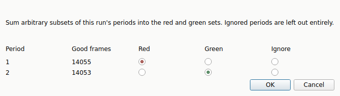
The Map Periods dialog for run 103277: period 1 assigned to Red, period 2 assigned to Green, each showing about 14,008 good frames. — The **Map Periods** dialog on run 103277. One row per period, each with its per-period **Good frames** count (≈ 14,008 here) and a three-way **Red** / **Green** / **Ignore** choice; **Ignore** drops a period from both sets. The defaults follow the photo-μSR convention — period 1 (laser ON) → **Red**, period 2 (laser OFF) → **Green**. For a plain two-period run the **RG Mode** radios in the grouping dialog already make this Red/Green choice directly; the mapping dialog comes into its own when a run holds more than two periods.

The scriptable API

The grouping controls call the same core period-selection API your scripts use, so the desktop app and a batch script agree on the per-period spectra. Pull out a single period as an ordinary MuonDataset:

from asymmetry.core.io import load, select_period, period_count, period_labels

run = load(".../Photo-muSR in silicon/Data/HIFI00103277.nxs")
print(period_count(run))                  # 2
print(period_labels(run))                 # ['red', 'green']

light_on = select_period(run, "red")      # period 1
light_off = select_period(run, "green")   # period 2

# ...or select a single period at load time:
light_off = load(
    ".../Data/HIFI00103277.nxs", period="green",
)

Each returned dataset keeps its parent’s \(t_0\), good-bin window, grouping, field, and temperature, plus its own per-period good_frames and dead_time_us. For files with three or more periods, pass a 1-based integer period number instead of a label.

Note

The convention here is laser-ON = Red (period 1) and laser-OFF = Green (period 2). It is worth confirming against the relaxation for your instrument and run before interpreting the difference — on run 103277 the check is unambiguous, since fitting each period gives \(\lambda \approx 1.3\;\mathrm{\mu s^{-1}}\) (strongly relaxing) for Red against \(\approx 0.09\;\mathrm{\mu s^{-1}}\) (near-flat) for Green.

Light on versus light off

The photo-μSR signal is the difference between the two periods: the laser-OFF period is the dark baseline, and the laser-ON period adds the extra relaxation from the photo-excited carriers. Overlaying the two asymmetries shows the effect by eye, with no fitting:

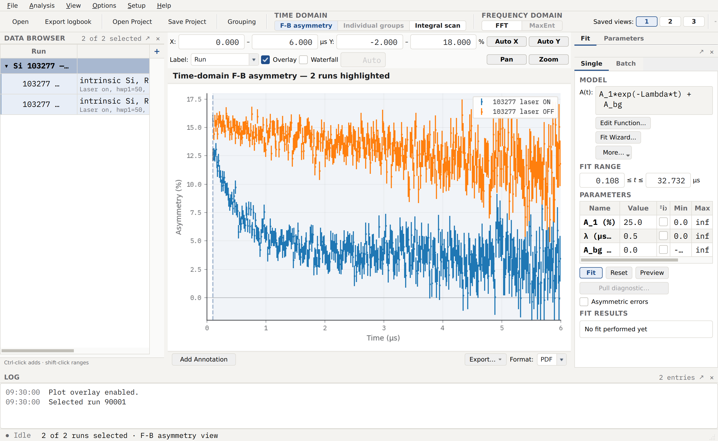
Time-domain asymmetry of run 103277 with the laser-ON and laser-OFF periods overlaid; the laser-ON trace relaxes strongly while the laser-OFF trace stays nearly flat. — Laser-ON (**Red** period, lower trace) and laser-OFF (**Green** period, upper trace) asymmetries of run 103277 overlaid over the first 6 μs, with the **Overlay** toolbar option enabled. The laser-OFF spectrum is near-flat — intrinsic silicon has little static relaxation in a small longitudinal field — while the laser-ON spectrum falls away over the first microsecond as the excess carriers depolarise the muonium. That extra relaxation is the observable; its rate \(\lambda\) is the carrier-density yardstick.

Extracting λ: the light-ON fit

The guide’s recipe fits each period with a single exponential \(A(t) = A_0\,e^{-\lambda t}\). Fit the laser-OFF period first with the amplitude free to obtain the baseline asymmetry \(A_0 \approx 15.5\%\); then refit the laser-ON period over the first 1 μs only, with \(A_0\) held fixed at that value, to read off \(\lambda\). The short window is deliberate — while the carriers are still present the density is essentially constant, so a single rate describes the decay (an assumption the lifetime below justifies).

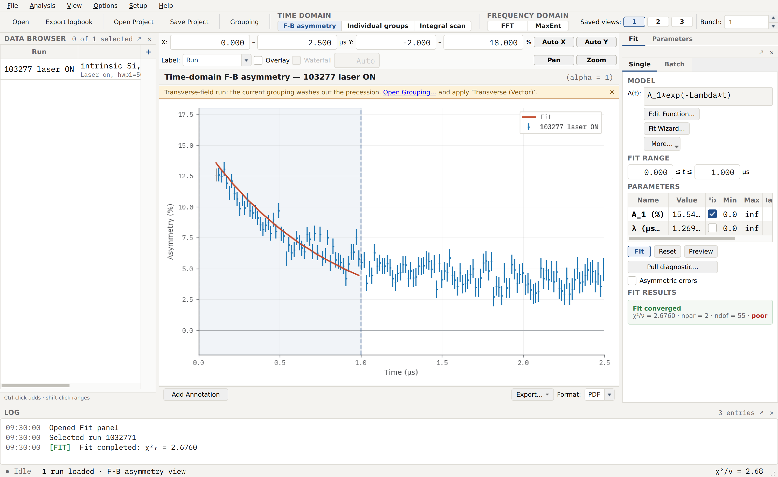
Single-exponential fit to the laser-ON period of run 103277 over the first microsecond, giving lambda about 1.27 per microsecond. — Single-exponential fit to the laser-ON period of the highest-density run 103277, restricted to the first 1 μs (shaded) with the amplitude fixed at the laser-OFF value. The rate comes out at \(\lambda = 1.27\;\mathrm{\mu s^{-1}}\), matching the digitised paper value (≈ 1.29). The fit is flagged **poor** (\(\chi^2/\nu \approx 2.7\)): a single exponential is a slight idealisation of a spectrum with more structure over 0–1 μs, but the recovered rate is robust. See Relaxation for the exponential relaxation component and Muonium for the underlying muonium dynamics.

Repeating this fit across the calibration set gives one \((\Delta n, \lambda)\) pair per run; across the delay scan it gives one \((\Delta T, \lambda)\) pair per run. The two trends that follow are built from those parameters.

Calibrating λ against Δn

For the calibration set the injected density \(\Delta n\) is known (it is the laser power the run was taken at), so plotting the fitted \(\lambda\) against \(\Delta n\) calibrates the yardstick. On log–log axes the relation is a power law,

\[\lambda = \beta \left(\frac{\Delta n}{\Delta n_0}\right)^{\alpha},\]

which appears as a straight line whose slope is the exponent \(\alpha\):

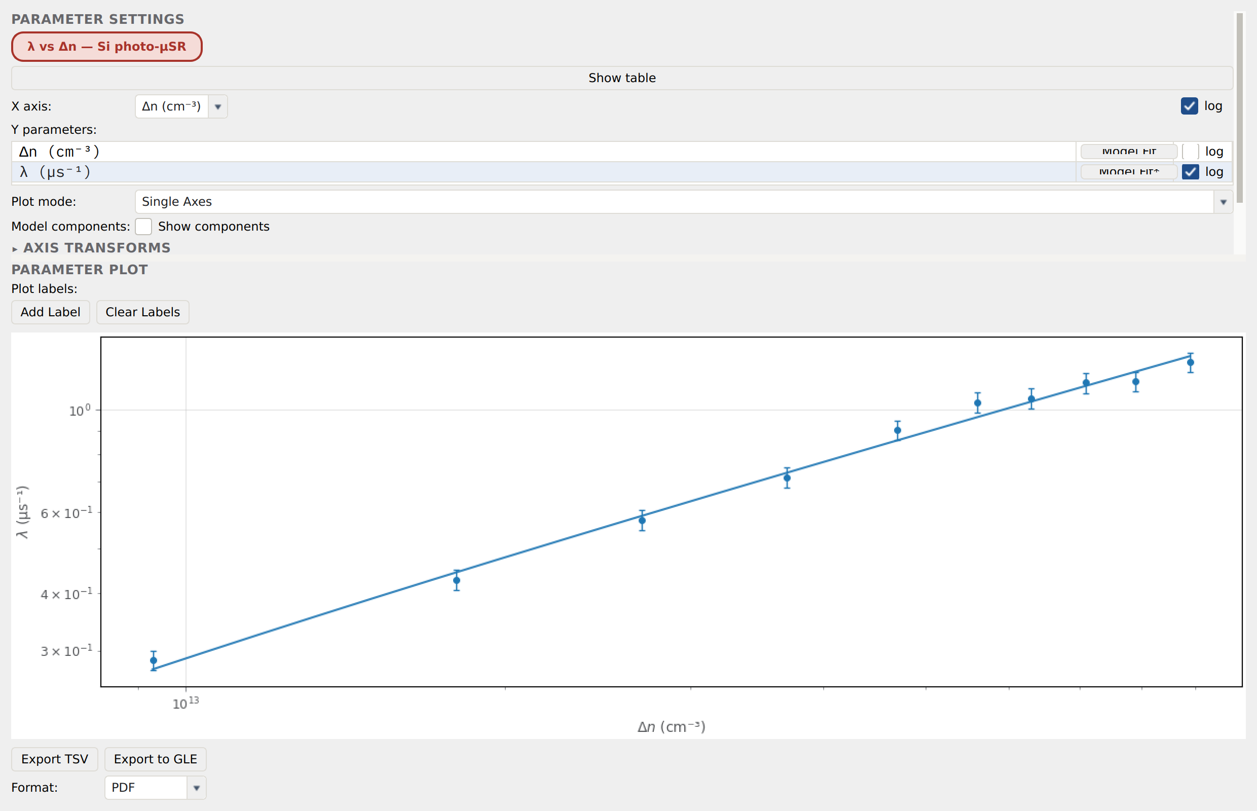
Log-log plot of relaxation rate lambda against excess carrier density delta n for the ten calibration runs, with a straight power-law fit through the points. — The **Fit Parameters** trending panel with \(\lambda\) on the y-axis against \(\Delta n\) on the x-axis, both on **log** scales, across the ten calibration runs (103277–103286). The power-law Model Fit* overlay is a straight line on these axes. The fitted exponent is \(\alpha = 0.65\), against the paper’s \(0.68(4)\) — within one standard deviation; the prefactor \(\beta = 1.30\;\mathrm{\mu s^{-1}}\) sits a little below the paper’s \(1.46(4)\), because the single-exponential rates run slightly low at small \(\Delta n\) (see the limitations below).

Inverting this calibration turns any measured \(\lambda\) back into a carrier density, which is exactly what the delay scan needs.

The headline: carrier lifetime τ₀

For the delay scan the injected density is fixed but the laser fires a delay \(\Delta T\) before the muon pulse, giving the carriers time to recombine. Fitting each run’s laser-ON \(\lambda\), inverting the calibration to a density, and plotting \(\Delta n\) against \(\Delta T\) traces the recombination directly. A single exponential \(\Delta n(\Delta T) = \Delta n(0)\,e^{-\Delta T / \tau_0}\) fits it, and \(\tau_0\) is the carrier recombination lifetime — the whole experiment’s primary deliverable:

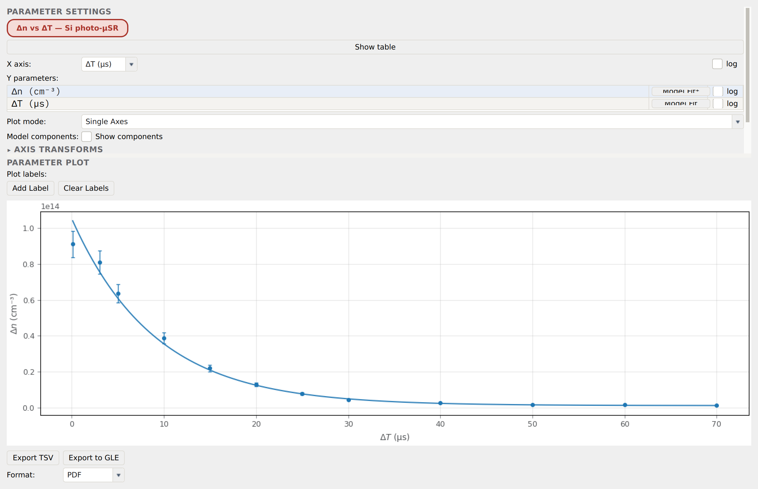
Excess carrier density delta n against laser delay delta T across the delay-scan runs, fitted with a single exponential decay giving a lifetime near 11 microseconds. — Excess carrier density \(\Delta n\) against laser delay \(\Delta T\) across the delay scan (runs 103287–103298), with the single-exponential Model Fit* overlay. The recovered lifetime is \(\tau_0 = 10.75\;\mathrm{\mu s}\), against the published \(11.1(9)\;\mathrm{\mu s}\) — agreement to within one standard deviation — and the fitted intercept \(\Delta n(0) \approx 9.8 \times 10^{13}\;\mathrm{cm^{-3}}\) matches the paper’s \(9.4(4) \times 10^{13}\). Because \(\tau_0 \gg 1\;\mathrm{\mu s}\), the density barely changes across the 1 μs fit window used for each \(\lambda\), which retrospectively justifies the constant-density assumption made when extracting the rates.

Assumptions and limitations

The analysis leans on a few deliberate simplifications, worth stating because they set the accuracy of the recovered numbers:

Single-exponential model, no baseline. Both the laser-OFF and laser-ON periods are fitted with a pure exponential and no constant term. This is the guide’s prescription and keeps the parameter count minimal, but the real laser-ON spectrum carries more structure than one exponential over 0–1 μs — hence the poor \(\chi^2/\nu \approx 2.7\) on the individual fit.
Amplitude fixed for the laser-ON fits. Holding \(A_0\) at the laser-OFF value removes a degeneracy between amplitude and rate in the short 1 μs window; it assumes the initial asymmetry is unchanged by the illumination.
Rates run low at low density. The fitted \(\lambda\) sit roughly 5–15 % below the digitised paper values at small \(\Delta n\), since a baseline-free single exponential underestimates a slow tail. This pulls the calibration exponent (\(\alpha = 0.65\) vs \(0.68(4)\)) and prefactor (\(\beta = 1.30\) vs \(1.46(4)\)) a little low. The headline \(\tau_0\) is insensitive to it, as it depends on the shape of \(\Delta n(\Delta T)\) rather than the calibration normalisation.
Default detector balance. The trends here use the loader’s default reduction (\(\alpha = 1\)); the transverse-field α calibration from run 103299 refines the absolute asymmetry but not the relaxation-rate ratios that drive the result. See EMU detector grouping and α calibration for the α-calibration workflow.

References

K. Yokoyama, J. S. Lord, J. Miao, P. Murahari, and A. J. Drew, Phys. Rev. Lett. 119, 226601 (2017) — the photoexcited-μSR carrier-lifetime method; the source of the calibration exponent \(\alpha = 0.68(4)\) and the lifetime \(\tau_0 = 11.1(9)\;\mathrm{\mu s}\) used as targets above. This example’s runs (RB1520457) are the same measurement.